Welcome to Shanshan Blog!

Classification comparasions in Scikit learn

2016-12-24

DataMining

Compare different Classification prediction result:


print(__doc__)

import numpy as np
import matplotlib.pyplot as plt
from matplotlib.colors import ListedColormap
from sklearn.model_selection import train_test_split
from sklearn.preprocessing import StandardScaler
from sklearn.datasets import make_moons, make_circles, make_classification
from sklearn.neural_network import MLPClassifier
from sklearn.neighbors import KNeighborsClassifier
from sklearn.svm import SVC
from sklearn.gaussian_process import GaussianProcessClassifier
from sklearn.gaussian_process.kernels import RBF
from sklearn.tree import DecisionTreeClassifier
from sklearn.ensemble import RandomForestClassifier, AdaBoostClassifier
from sklearn.naive_bayes import GaussianNB
from sklearn.discriminant_analysis import QuadraticDiscriminantAnalysis

h = .02  # step size in the mesh

names = ["Nearest Neighbors", "Linear SVM", "RBF SVM", "Gaussian Process",
         "Decision Tree", "Random Forest", "Neural Net", "AdaBoost",
         "Naive Bayes", "QDA"]

classifiers = [
    KNeighborsClassifier(3),
    SVC(kernel="linear", C=0.025),
    SVC(gamma=2, C=1),
    GaussianProcessClassifier(1.0 * RBF(1.0), warm_start=True),
    DecisionTreeClassifier(max_depth=5),
    RandomForestClassifier(max_depth=5, n_estimators=10, max_features=1),
    MLPClassifier(alpha=1),
    AdaBoostClassifier(),
    GaussianNB(),
    QuadraticDiscriminantAnalysis()]

X, y = make_classification(n_features=2, n_redundant=0, n_informative=2,
                           random_state=1, n_clusters_per_class=1)
rng = np.random.RandomState(2)
X += 2 * rng.uniform(size=X.shape)
linearly_separable = (X, y)

datasets = [make_moons(noise=0.3, random_state=0),
            make_circles(noise=0.2, factor=0.5, random_state=1),
            linearly_separable
            ]

figure = plt.figure(figsize=(27, 9))
i = 1
# iterate over datasets
for ds_cnt, ds in enumerate(datasets):
    # preprocess dataset, split into training and test part
    X, y = ds
    X = StandardScaler().fit_transform(X)
    X_train, X_test, y_train, y_test = \
        train_test_split(X, y, test_size=.4, random_state=42)

    x_min, x_max = X[:, 0].min() - .5, X[:, 0].max() + .5
    y_min, y_max = X[:, 1].min() - .5, X[:, 1].max() + .5
    xx, yy = np.meshgrid(np.arange(x_min, x_max, h),
                         np.arange(y_min, y_max, h))

    # just plot the dataset first
    cm = plt.cm.RdBu
    cm_bright = ListedColormap(['#FF0000', '#0000FF'])
    ax = plt.subplot(len(datasets), len(classifiers) + 1, i)
    if ds_cnt == 0:
        ax.set_title("Input data")
    # Plot the training points
    ax.scatter(X_train[:, 0], X_train[:, 1], c=y_train, cmap=cm_bright)
    # and testing points
    ax.scatter(X_test[:, 0], X_test[:, 1], c=y_test, cmap=cm_bright, alpha=0.6)
    ax.set_xlim(xx.min(), xx.max())
    ax.set_ylim(yy.min(), yy.max())
    ax.set_xticks(())
    ax.set_yticks(())
    i += 1

    # iterate over classifiers
    for name, clf in zip(names, classifiers):
        ax = plt.subplot(len(datasets), len(classifiers) + 1, i)
        clf.fit(X_train, y_train)
        score = clf.score(X_test, y_test)

        # Plot the decision boundary. For that, we will assign a color to each
        # point in the mesh [x_min, x_max]x[y_min, y_max].
        if hasattr(clf, "decision_function"):
            Z = clf.decision_function(np.c_[xx.ravel(), yy.ravel()])
        else:
            Z = clf.predict_proba(np.c_[xx.ravel(), yy.ravel()])[:, 1]

        # Put the result into a color plot
        Z = Z.reshape(xx.shape)
        ax.contourf(xx, yy, Z, cmap=cm, alpha=.8)

        # Plot also the training points
        ax.scatter(X_train[:, 0], X_train[:, 1], c=y_train, cmap=cm_bright)
        # and testing points
        ax.scatter(X_test[:, 0], X_test[:, 1], c=y_test, cmap=cm_bright,
                   alpha=0.6)

        ax.set_xlim(xx.min(), xx.max())
        ax.set_ylim(yy.min(), yy.max())
        ax.set_xticks(())
        ax.set_yticks(())
        if ds_cnt == 0:
            ax.set_title(name)
        ax.text(xx.max() - .3, yy.min() + .3, ('%.2f' % score).lstrip('0'),
                size=15, horizontalalignment='right')
        i += 1

plt.tight_layout()
plt.show()

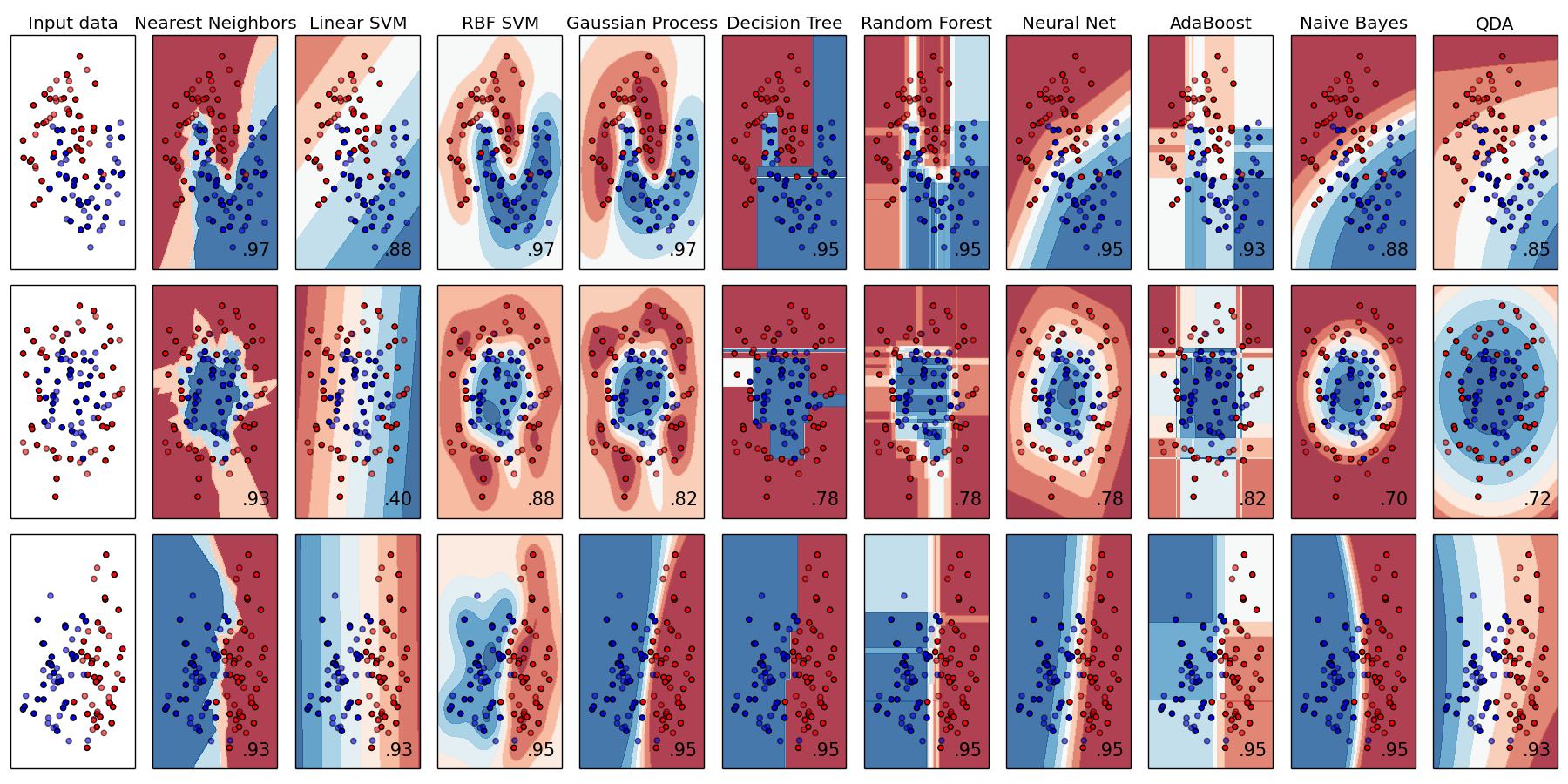
The result is:

Read All

KNN Review

2016-12-22

DataMining

DataMining
KNN Review

What is KNN (K-Nearest Neighbors Algorithm)

K Nearest Neighbor is one of classification algorithms that are very simple to understand but works incredibly well in practice. In pattern recognition, the k-Nearest Neighbors algorithm is a non-parametric method used for classification and regression [1]. In both cases, the input consists of the k closest training examples in the feature space.

When a prediction is required for a unseen data instance, the KNN algorithm will search through the training dataset for the k-most similar instances. The prediction attribute of the most similar instances is summarized and returned as the prediction for the unseen instance.

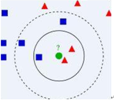
Take a simple example to describe it:

In Figure 1, there are two type data, including blue diamond and red triangle. Assume that our task is to find which class the green data belong to. How do we do it? Assume that only the nearest ones are helpful to find its classification. But how many objects to determine it? If k = 3 (solid line circle) it is assigned to the second class because there are 2 triangles and only 1 square inside the inner circle. If k = 5 (dashed line circle) it is assigned to the first class (3 squares vs. 2 triangles inside the outer circle).

How to Compute KNN Algorithm
```
Step 1: Calculate the distances between the current node and the nodes in the dataset

Step 2: Sort all the distances

Step 3: Choose the minimum K distance

Step 4: Return the classification with the highest frequency
```
Distance Calculation

Often, the classification accuracy of KNN can be improved significantly if the distance metric is learned with specialized algorithms such as Large Margin Nearest Neighbor [2] or Neighborhood components analysis [3]. Euclidean metric is the most popular choice for the distance function. If the measurement variables are not of comparable units and scales, it is more meaningful to standardize the variables before using the Euclidean distance for classification.

If an estimate of the pooled dispersion matrix is used for standardization, it essentially leads to classification using Mahalanobis distances [12]. And many other flexible metrics can be used as well [15, 16].

How to Choose K (Neighbors)

Performance of a nearest neighbor classifier depends on the distance function and the value of the neighborhood parameter k. The neighborhood parameter k, which controls the volume of the neighborhood and consequently the smoothness of the density estimates, plays an important role on the performance of a nearest neighbor classifier.

Existing theoretical results [8, 1] suggest that if Euclidean distance is used for classification, one should vary k with n in such a way that and as . The same assertion holds also for Mahalanobis distance if one uses any consistent estimate of the pooled dispersion matrix for standardization. However, for small or moderately large sample sizes, there is no theoretical guideline for choosing the optimum value of k. This optimum value depends on the specific data set and it is to be estimated using the available training sample observations.

In practice, one uses cross-validation methods [9, 10] to estimate the misclassification rate for different values of k and chooses that one which leads to the lowest estimate of misclassification rate. However, these cross-validation techniques use naive empirical proportions for estimating the misclassification probabilities. As a consequence, multiple values of k as minimizers of estimated misclassification rate, is difficult to choose the optimum one. Ghosh and Chaudhuri [11] proposed a smooth estimate for the misclassification probability function for finding the optimal bandwidth parameter.

Weight

Usually, uniform weights are used in K-Nearest Neighbor Algorithm. In other words, all points in each neighborhood are weighted equally. It takes the assumption that training data are evenly distributed among all categories. However, there is no guarantee that training set is balanced populated.

As an improvement to KNN, distance-weighted KNN method was introduced that closer neighbors of a query point will have a greater influence than neighbors which are further away. Dudani introduced a distance-weighted KNN rule (WKNN) with the basic idea of weighting close neighbors more heavily, according to their distances to the query [4]. Songbo Tan proposed Neighbor-Weighted K-Nearest Neighbor (NWKNN) for unbalanced text categorization problems. NWKNN assigns a big weight for neighbors from small class, and assigns a little weight for neighbors contained in large category [5].

Another popular framework is Voting method [6], which combines the predictions of multiple same classifiers to boost classification accuracy. Voting algorithms can be divided into two types: Bagging and Boosting. The main difference between the two types is the way the different versions of the training set are created. Bagging use a uniform probability to select a new training set while Boosting according to how often one example was misclassified by previous classifiers to select one example to create a new training set [7].

Algorithm

Advanced Improvement

Improvement Summary

Test Data: Iris Plants Database (From Python Package) Base data: [‘sepal length (cm)’, ‘sepal width (cm)’, ‘petal length (cm)’, ‘petal width (cm)’] – Four Features Target: [‘setosa’, ‘versicolor’, ‘virginica’] – Three Type Iris Plants Number of Instances: 150 (50 in each of three classes)

Reference

[1] Cover T, Hart P. Nearest neighbor pattern classification[J]. IEEE transactions on information theory, 1967, 13(1): 21-27.

[2] Weinberger K Q, Blitzer J, Saul L K. Distance metric learning for large margin nearest neighbor classification[C]//Advances in neural information processing systems. 2005: 1473-1480.

[3] Goldberger J, Hinton G E, Roweis S T, et al. Neighbourhood components analysis[C]//Advances in neural information processing systems. 2004: 513-520.

[4] Dudani S A. The distance-weighted k-nearest-neighbor rule[J]. IEEE Transactions on Systems, Man, and Cybernetics, 1976 (4): 325-327.

[5] Tan S. Neighbor-weighted k-nearest neighbor for unbalanced text corpus[J]. Expert Systems with Applications, 2005, 28(4): 667-671.

[6] Sebastiani F. Machine learning in automated text categorization[J]. ACM computing surveys (CSUR), 2002, 34(1): 1-47.

[7] Tan S. An effective refinement strategy for KNN text classifier[J]. Expert Systems with Applications, 2006, 30(2): 290-298.

[8] Loftsgaarden D O, Quesenberry C P. A nonparametric estimate of a multivariate density function[J]. The Annals of Mathematical Statistics, 1965, 36(3): 1049-1051.

[9] Lachenbruch P A, Mickey M R. Estimation of error rates in discriminant analysis[J]. Technometrics, 1968, 10(1): 1-11.

[10] Stone M. Cross-validation: a review 2[J]. Statistics: A Journal of Theoretical and Applied Statistics, 1978, 9(1): 127-139.

[11] Ghosh A K, Chaudhuri P. Optimal smoothing in kernel discriminant analysis[J]. Statistica Sinica, 2004: 457-483.

[12] Mahalanobis P C. On the generalized distance in statistics[J]. Proceedings of the National Institute of Sciences (Calcutta), 1936, 2: 49-55.

[13] Friedman J H. Flexible metric nearest neighbor classification[R]. Technical report, Department of Statistics, Stanford University, 1994.

[14] Hastie T, Tibshirani R. Discriminant adaptive nearest neighbor classification[J]. IEEE transactions on pattern analysis and machine intelligence, 1996, 18(6): 607-616.

[15] Friedman J H. Flexible metric nearest neighbor classification[R]. Technical report, Department of Statistics, Stanford University, 1994.

[16] Hastie T, Tibshirani R. Discriminant adaptive nearest neighbor classification[J]. IEEE transactions on pattern analysis and machine intelligence, 1996, 18(6): 607-616.

[17] Cover T, Hart P. Nearest neighbor pattern classification[J]. IEEE transactions on information theory, 1967, 13(1): 21-27.
Read All
Classification vs Clustering

2016-12-21

DataMining

DataMining
Classification - the task of assigning instances to pre-defined classes.
- e.g. Deciding whether a particular patient record can be associated with a specifit disease.
Clustering - the task of grouping related data points together without labeling them.
- e.g. Grouping patient records with similiar symptoms without knowing what the symptoms indicate.
Read All

Python files and folders movement

2016-12-20

Python

To move the files to the folders, prefix of files’name is same as the folder. For example, “table_test.csv” move to folder “table”.

import os
import shutil
import sys
reload(sys)
sys.setdefaulutencoding("utf-8")

os.environ['NLS_LANG'] = 'SIMPLIFIED CHINESE_CHINA.UTF8'

# direction with all the fiels going to move
dir = os.path.join(os.path.dirname(__file__), u'D:/AllFiles') # or use .decode('utf-8')
print dir

pathDir = os.listdir(dir)

fns = [os.path.join(dir, fn) for parent, dirnames, filenames in os.walk(dir) for fn in filenames]
str = 'D:/ 空文件夹/'
for f in fns:
    temp = f[18: len(f)].split("_")[0]
    str = 'D:/ 空文件夹/' + temp
    # if the folder exists, move to it, else print the file
    if (os.path.exists(str)):
        shutil.move(f, str.decode('utf-8'))
    else:
        print f

Read All

Compare cross decomposition methods in Python

2016-12-19

DataMining

Data Mining python

The cross decomposition module contains two main families of algorithms: the partial least squares (PLS) and the canonical correlation analysis (CCA).

Compare PLS and CCA.

import numpy as np
import matplotlib.pyplot as plt
from sklearn.cross_decomposition import PLSCanonical, PLSRegression, CCA

n = 500
# get the random array, 2 latents vars:
l1 = np.random.normal(size=n)
l2 = np.random.normal(size=n)

latents = np.array([l1, l1, l2, l2]).T
X = latents + np.random.normal(size=4 * n).reshape((n, 4))
Y = latents + np.random.normal(size=4 * n).reshape((n, 4))

X_train = X[:n / 2]
Y_train = Y[:n / 2]
X_test = X[n / 2:]
Y_test = Y[n / 2:]

# correlation coefficients
print("Corr(X)")
print(np.round(np.corrcoef(X.T), 2))
print("Corr(Y)")
print(np.round(np.corrcoef(Y.T), 2))

###############################################################################
# Canonical (symmetric) PLS
# Partial Least Squares 偏最小二乘法
# Transform data
# ~~~~~~~~~~~~~~
plsca = PLSCanonical(n_components=2)
plsca.fit(X_train, Y_train)
X_train_r, Y_train_r = plsca.transform(X_train, Y_train)
X_test_r, Y_test_r = plsca.transform(X_test, Y_test)

# Scatter plot of scores
# ~~~~~~~~~~~~~~~~~~~~~~
# 1) On diagonal plot X vs Y scores on each components
plt.figure(figsize=(12, 8))
plt.subplot(221)
plt.plot(X_train_r[:, 0], Y_train_r[:, 0], "ob", label="train")
plt.plot(X_test_r[:, 0], Y_test_r[:, 0], "or", label="test")
plt.xlabel("x scores")
plt.ylabel("y scores")
plt.title('Comp. 1: X vs Y (test corr = %.2f)' %
          np.corrcoef(X_test_r[:, 0], Y_test_r[:, 0])[0, 1])
plt.xticks(())
plt.yticks(())
plt.legend(loc="best")

plt.subplot(224)
plt.plot(X_train_r[:, 1], Y_train_r[:, 1], "ob", label="train")
plt.plot(X_test_r[:, 1], Y_test_r[:, 1], "or", label="test")
plt.xlabel("x scores")
plt.ylabel("y scores")
plt.title('Comp. 2: X vs Y (test corr = %.2f)' %
          np.corrcoef(X_test_r[:, 1], Y_test_r[:, 1])[0, 1])
plt.xticks(())
plt.yticks(())
plt.legend(loc="best")

# 2) Off diagonal plot components 1 vs 2 for X and Y
plt.subplot(222)
plt.plot(X_train_r[:, 0], X_train_r[:, 1], "*b", label="train")
plt.plot(X_test_r[:, 0], X_test_r[:, 1], "*r", label="test")
plt.xlabel("X comp. 1")
plt.ylabel("X comp. 2")
plt.title('X comp. 1 vs X comp. 2 (test corr = %.2f)'
          % np.corrcoef(X_test_r[:, 0], X_test_r[:, 1])[0, 1])
plt.legend(loc="best")
plt.xticks(())
plt.yticks(())

plt.subplot(223)
plt.plot(Y_train_r[:, 0], Y_train_r[:, 1], "*b", label="train")
plt.plot(Y_test_r[:, 0], Y_test_r[:, 1], "*r", label="test")
plt.xlabel("Y comp. 1")
plt.ylabel("Y comp. 2")
plt.title('Y comp. 1 vs Y comp. 2 , (test corr = %.2f)'
          % np.corrcoef(Y_test_r[:, 0], Y_test_r[:, 1])[0, 1])
plt.legend(loc="best")
plt.xticks(())
plt.yticks(())
plt.show()

###############################################################################
# PLS regression, with multivariate response, a.k.a. PLS2

n = 1000
q = 3
p = 10
X = np.random.normal(size=n * p).reshape((n, p))
B = np.array([[1, 2] + [0] * (p - 2)] * q).T
# each Yj = 1*X1 + 2*X2 + noize
Y = np.dot(X, B) + np.random.normal(size=n * q).reshape((n, q)) + 5

pls2 = PLSRegression(n_components=3)
pls2.fit(X, Y)
print("True B (such that: Y = XB + Err)")
print(B)
# compare pls2.coef_ with B
print("Estimated B")
print(np.round(pls2.coef_, 1))
pls2.predict(X)

###############################################################################
# PLS regression, with univariate response, a.k.a. PLS1

n = 1000
p = 10
X = np.random.normal(size=n * p).reshape((n, p))
y = X[:, 0] + 2 * X[:, 1] + np.random.normal(size=n * 1) + 5
pls1 = PLSRegression(n_components=3)
pls1.fit(X, y)
# note that the number of components exceeds 1 (the dimension of y)
print("Estimated betas")
print(np.round(pls1.coef_, 1))

###############################################################################
# CCA (PLS mode B with symmetric deflation)

cca = CCA(n_components=2)
cca.fit(X_train, Y_train)
X_train_r, Y_train_r = plsca.transform(X_train, Y_train)
X_test_r, Y_test_r = plsca.transform(X_test, Y_test)

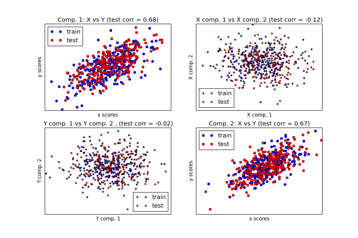
The result is:

Read All

Python connects with SQL

2016-12-15

SQL

SQL Python

Python connect with SQL to get the sql query result.

import psycopg2
import sys
import pandas as pd
from sqlalchemy import create_engine
import os
import sqlalchemy

# pgSQL
engine1 = create_engine('postgresql+psycopg2://...') # including the sql username and password
# if connect with Oracle, for Chinese
os.environ['NLS_LANG'] = 'SIMPLIFIED CHINESE_CHINA.UTF8'

sql = "SQL QUERY LIKE SELECT ..."
# sometimes it may occur the situation:  sql 含转义字符, add one more line
sql = sqlalchemy.text(sql)
df = pd.read_sql_query(sql.engine1)
# df is the result of sql query
# pgSQL Chinese is fine, but for the Oracle or mySQL, it maybe be wrong, add one line
# for the chinese columns
name = name.encode('latin-1').decode('gbk')

Read All

21/38

Welcome to Shanshan Blog!

Classification comparasions in Scikit learn

KNN Review

What is KNN (K-Nearest Neighbors Algorithm)

How to Compute KNN Algorithm

Distance Calculation

How to Choose K (Neighbors)

Weight

Algorithm

Improvement Summary

Reference

Classification vs Clustering

Python files and folders movement

Compare cross decomposition methods in Python

Python connects with SQL