Welcome to Shanshan Blog!
-
Update all Python Packages in one time
import pip
from subprocess import call

for dist in pip.get_installed_distributions():
    call("pip install --upgrade " + dist.project_name, shell=True)
-
Model Selection in Python
Cross validation is a model evaluation method that is better than residuals. The problem with residual evaluations is that they do not give an indication of how well the learner will do when it is asked to make new predictions for data it has not already seen. One way to overcome this problem is to not use the entire data set when training a learner. Some of the data is removed before training begins. Then when training is done, the data that was removed can be used to test the performance of the learned model on new data. This is the basic idea for a whole class of model evaluation methods called cross validation.
Data and model preparation:
import numpy as np from sklearn.model_selection import train_test_split from sklearn import datasets from sklearn import svm iris = datasets.load_iris() X_train, X_test, y_train, y_test = train_test_split(iris.data, iris.target, test_size=0.4, random_state=0) clf = svm.SVC(kernel='linear', C= 1).fit(X_train, y_train)- Hold-Out Method
The holdout method is the simplest kind of cross validation. The data set is separated into two sets, called the training set and the testing set. The function approximator fits a function using the training set only. Then the function approximator is asked to predict the output values for the data in the testing set. The errors it makes are accumulated as before to give the mean absolute test set error, which is used to evaluate the model. The advantage of this method is that it is usually preferable to the residual method and takes no longer to compute. However, its evaluation can have a high variance.
- K-fold cross validation
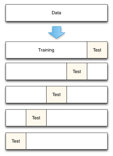
K-fold cross validation is one way to improve over the holdout method. The data set is divided into k subsets, and the holdout method is repeated k times. Each time, one of the k subsets is used as the test set and the other k-1 subsets are put together to form a training set. Then the average error across all k trials is computed. The advantage of this method is that it matters less how the data gets divided. Every data point gets to be in a test set exactly once, and gets to be in a training set k-1 times. The variance of the resulting estimate is reduced as k is increased. The disadvantage of this method is that the training algorithm has to be rerun from scratch k times, which means it takes k times as much computation to make an evaluation.

# k-folder cross validation
scores = cross_val_score(clf, iris.data, iris.target, cv=5)
print scores
The output is:
[ 0.96666667 1. 0.96666667 0.96666667 1. ]
Accuracy: 0.98 (+/- 0.03)
- Cross validation iterators
K Folder
KFold divides all the samples in k groups of samples, called folds (if k = n, this is equivalent to the Leave One Out strategy), of equal sizes (if possible). The prediction function is learned using k - 1 folds, and the fold left out is used for test.
# k folder
X = ["a", "b", "c", "d"]
from sklearn.model_selection import KFold
kf = KFold(n_splits=2)
for train, test in kf.split(X):
    print ("%s %s" % (train, test))
# Each fold is constituted by two arrays: the first one is related to the training set, and the second one to the test set.
X = np.array([[0., 0.], [1., 1.], [-1., -1.], [2., 2.]])
y = np.array([0, 1, 0, 1])
X_train, X_test, y_train, y_test = X[train], X[test], y[train], y[test]
print X_train
Leave One Out
Each learning set is created by taking all the samples except one, the test set being the sample left out. Thus, for n samples, we have n different training sets and n different tests set. This cross-validation procedure does not waste much data as only one sample is removed from the training set:
# leave out
from sklearn.model_selection import LeavePOut
X = np.ones(4)
lpo = LeavePOut(p = 2)
for train, test in lpo.split(X):
    print("%s %s" % (train, test))
-
Oversample Method SMOTE
Over-sampling with replacement and has noted that it doesn’t significantly improve minority class recognition. Chawla proposed an over-sampling approach in which the minority class is over-sampled by creating “synthetic” examples rather than by over-sampling with replacement.
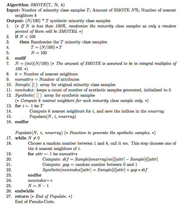
They generate synthetic examples in a less application-specific manner, by operating in “feature space” rather than “data space”. The minority class is over-sampled by taking each minority class sample and introducing synthetic examples along the line segments joining any/all of the k minority class nearest neighbors. Depending upon the amount of over-sampling required, neighbors from the k nearest neighbors are randomly chosen.
Its pseudo-code is :

In python package imbalanced-learn, this method can be achieved.
imblearn.over_sampling.SMOTE
import matplotlib.pyplot as plt
import seaborn as sns
from sklearn.datasets import make_classification
from sklearn.decomposition import PCA

from imblearn.over_sampling import SMOTE

print(__doc__)

sns.set()

# Define some color for the plotting
almost_black = '#262626'
palette = sns.color_palette()


# Generate the dataset
X, y = make_classification(n_classes=2, class_sep=2, weights=[0.1, 0.9],
                           n_informative=3, n_redundant=1, flip_y=0,
                           n_features=20, n_clusters_per_class=1,
                           n_samples=5000, random_state=10)

# Instanciate a PCA object for the sake of easy visualisation
pca = PCA(n_components=2)
# Fit and transform x to visualise inside a 2D feature space
X_vis = pca.fit_transform(X)

# Apply regular SMOTE
sm = SMOTE(kind='regular')
X_resampled, y_resampled = sm.fit_sample(X, y)
X_res_vis = pca.transform(X_resampled)

# Two subplots, unpack the axes array immediately
f, (ax1, ax2) = plt.subplots(1, 2)

ax1.scatter(X_vis[y == 0, 0], X_vis[y == 0, 1], label="Class #0", alpha=0.5,
            edgecolor=almost_black, facecolor=palette[0], linewidth=0.15)
ax1.scatter(X_vis[y == 1, 0], X_vis[y == 1, 1], label="Class #1", alpha=0.5,
            edgecolor=almost_black, facecolor=palette[2], linewidth=0.15)
ax1.set_title('Original set')

ax2.scatter(X_res_vis[y_resampled == 0, 0], X_res_vis[y_resampled == 0, 1],
            label="Class #0", alpha=.5, edgecolor=almost_black,
            facecolor=palette[0], linewidth=0.15)
ax2.scatter(X_res_vis[y_resampled == 1, 0], X_res_vis[y_resampled == 1, 1],
            label="Class #1", alpha=.5, edgecolor=almost_black,
            facecolor=palette[2], linewidth=0.15)
ax2.set_title('SMOTE regular')

plt.show()
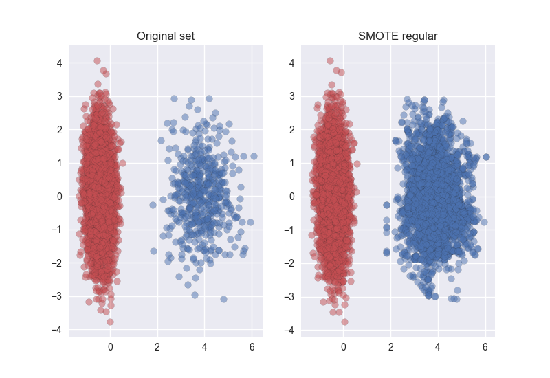
The result is:

More SMOTE Improvement methods can be got here imblearn.over_sampling.SMOTE
You can get the paper for this method here: SMOTE: Synthetic Minority Over-sampling Technique
-
Undersample Methods in Python
balanced-learn package offers some under-sampling methods:
-
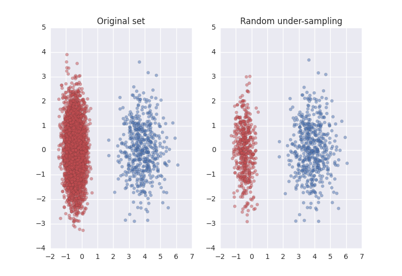
Random majority under-sampling with replacement
-
Extraction of majority-minority Tomek links [1]
-
Under-sampling with Cluster Centroids
-
NearMiss-(1 & 2 & 3) [2]
-
Condensend Nearest Neighbour [3]
-
One-Sided Selection [4]
-
Neighboorhood Cleaning Rule [5]
-
Edited Nearest Neighbours [6]
-
Instance Hardness Threshold [7]
-
Repeated Edited Nearest Neighbours [14]
-
AllKNN [14]
Random under-sample in python
import matplotlib.pyplot as plt
import seaborn as sns
from sklearn.datasets import make_classification
from sklearn.decomposition import PCA

from imblearn.under_sampling import RandomUnderSampler

sns.set()

# Define some color for the plotting
almost_black = '#262626'
palette = sns.color_palette()


# Generate the dataset
X, y = make_classification(n_classes=2, class_sep=2, weights=[0.1, 0.9],
                           n_informative=3, n_redundant=1, flip_y=0,
                           n_features=20, n_clusters_per_class=1,
                           n_samples=5000, random_state=10)

# Instanciate a PCA object for the sake of easy visualisation
pca = PCA(n_components=2)
# Fit and transform x to visualise inside a 2D feature space
X_vis = pca.fit_transform(X)

# Apply the random under-sampling
rus = RandomUnderSampler()
X_resampled, y_resampled = rus.fit_sample(X, y)
X_res_vis = pca.transform(X_resampled)

# Two subplots, unpack the axes array immediately
f, (ax1, ax2) = plt.subplots(1, 2)

ax1.scatter(X_vis[y == 0, 0], X_vis[y == 0, 1], label="Class #0", alpha=0.5,
            edgecolor=almost_black, facecolor=palette[0], linewidth=0.15)
ax1.scatter(X_vis[y == 1, 0], X_vis[y == 1, 1], label="Class #1", alpha=0.5,
            edgecolor=almost_black, facecolor=palette[2], linewidth=0.15)
ax1.set_title('Original set')

ax2.scatter(X_res_vis[y_resampled == 0, 0], X_res_vis[y_resampled == 0, 1],
            label="Class #0", alpha=.5, edgecolor=almost_black,
            facecolor=palette[0], linewidth=0.15)
ax2.scatter(X_res_vis[y_resampled == 1, 0], X_res_vis[y_resampled == 1, 1],
            label="Class #1", alpha=.5, edgecolor=almost_black,
            facecolor=palette[2], linewidth=0.15)
ax2.set_title('Random under-sampling')

plt.show()
-
-
Class Imbalance
Class Imbalance Problem
It is the problem in machine learning where the total number of a class of data (positive) is far less than the total number of another class of data
Oversampling and undersampling in data analysis are techniques used to adjust the class distribution of a dataset.
Why is it a problem?
Most machine learning algorithms and works best when the number of instances of each classes are roughly equal. When the number of instances of one class far exceeds the other, problems arise.
How to deal with this problem?
Cost function based approaches
The intuition behind cost function based approaches is that if we think one false negative is worse than one false positive, we will count that one false negative as, e.g., 100 false negatives instead.
Sampling based approaches
This can be roughly classified into three categories:
-
Oversampling, by adding more of the minority class so it has more effect on the machine learning algorithm
-
Undersampling, by removing some of the majority class so it has less effect on the machine learning algorithm
-
Hybrid, a mix of oversampling and undersampling
-
-
Python OS File Operations
Open the file for writing and reading.
import os

input = open(filename, 'r')	# read
output = open(filename, 'w') # write
output = open(filename, 'a') # write more
Walk the whole folder
for root, dirs, files in os.walk(path, topdown=False):
	#hanlde file
	for name in files:
		if name[:-3] = 'exe':
		print name
Delete Files
top='mydata/'
for root,dir,files in os.walk(top,topdown=False):
      for name in files:
     os.remove(os.path.join(root,name))

os.rmdir('mydata')
os.mkdir('mydata')