Welcome to Shanshan Blog!
-
Data Mining Proprocessing in Python Standardization and Normalization
- Standardization
- Scaling features to a range
- Scaling sparse data
- Scaling data with outliers
- Normalization
The sklearn.preprocessing package provides several common utility functions and transformer classes.
Standardization
Centering and scaling happen independently on each feature by computing the relevant statistics on the samples in the training set. Mean and standard deviation are then stored to be used on later data using the transform method.
In practice we often ignore the shape of the distribution and just transform the data to center it by removing the mean value of each feature, then scale it by dividing non-constant features by their standard deviation.
# scale : quick to do standarization
x = np.array([[ 1., -1.,  2.],
              [ 2.,  0.,  0.],
              [ 0.,  1., -1.]])
x_scale = preprocessing.scale(x)
print x_scale
# scale data has zero means and unit variance
print "Scale mean is \n", x_scale.mean(axis = 0)
print "Scale std is \n",x_scale.std(axis = 0)
The output is
	[[ 0.         -1.22474487  1.33630621]
	 [ 1.22474487  0.         -0.26726124]
	 [-1.22474487  1.22474487 -1.06904497]]
	Scale mean is
	[ 0.  0.  0.]
	Scale std is
	[ 1.  1.  1.]
sklearn also provides sklearn.preprocessing.StandardScaler to compute the mean and standard deviation on a training set in case that training data uses the same transformation.
sklearn.preprocessing.StandardScaler(copy=True, with_mean=True, with_std=True)
with_mean: If True, center the data before scaling.

with_str: If True, scale the data to unit variance.

copy: If False, try to avoid a copy and do inplace scaling instead.
Attributes:
scale_

mean_

var_

n_samples_seen_: The number of samples processed by the estimator.
StandardScaler Examples
# sklearn.preprocessing.StandardScaler
scaler = preprocessing.StandardScaler().fit(x)

print "Mean is \n", scaler.mean_
print "Std is \n", scaler.std_
print "Scale is \n", scaler.scale_
print scaler.transform(x)
The output is
	Mean is
	[ 1.          0.          0.33333333]
	Std is
	[ 0.81649658  0.81649658  1.24721913]
	Scale is
	[ 0.81649658  0.81649658  1.24721913]
	[[ 0.         -1.22474487  1.33630621]
	 [ 1.22474487  0.         -0.26726124]
	 [-1.22474487  1.22474487 -1.06904497]]
Scaling features to a range
An alternative standardization is scaling features to lie between a given minimum and maximum value. This can be achieved using MinMaxScaler or MaxAbsScaler, respectively.
MinMaxScaler transformation formula:
X_std = (X - X.min(axis=0)) / (X.max(axis=0) - X.min(axis=0))
X_scaled = X_std * (max - min) + min
sklearn.preprocessing.MinMaxScaler(feature_range=(0, 1), copy=True)[source]
Attributes: min_, scale_, data_min_, data_max_, data_range_
min_max_scaler = preprocessing.MinMaxScaler()
x_minmax = min_max_scaler.fit_transform(x)
print x_minmax
print "min_max_scaler scale is \n", x_minmax.scale_
print "min_max_scaler min is \n", x_minmax.min_
The output is
	[[ 0.5         0.          1.        ]
	 [ 1.          0.5         0.33333333]
	 [ 0.          1.          0.        ]]
	min_max_scaler scale is
	[ 0.5         0.5         0.33333333]
	min_max_scaler min is
	[ 0.          0.5         0.33333333]
MaxAbsScaler works in a very similar fashion, but scales in a way that the training data lies within the range [-1, 1] by dividing through the largest maximum value in each feature. It is meant for data that is already centered at zero or sparse data.
sklearn.preprocessing.MaxAbsScaler(copy=True)
MaxAbsScaler
max_abs_scaler = preprocessing.MaxAbsScaler()
x_maxabs = max_abs_scaler.fit_transform(x)
print x_maxabs
print max_abs_scaler.scale_
Scaling sparse data
Centering sparse data would destroy the sparseness structure in the data, and thus rarely is a sensible thing to do. However, it can make sense to scale sparse inputs, especially if features are on different scales.
MaxAbsScaler and maxabs_scale were specifically designed for scaling sparse data, and are the recommended way to go about this. However, scale and StandardScaler can accept scipy.sparse matrices as input, as long as with_mean=False is explicitly passed to the constructor.
Scaling data with outliers
If your data contains many outliers, scaling using the mean and variance of the data is likely to not work very well. In these cases, you can use robust_scale and RobustScaler as drop-in replacements instead. They use more robust estimates for the center and range of your data.
sklearn.preprocessing.robust_scale(X, axis=0, with_centering=True, with_scaling=True, quantile_range=(25.0, 75.0), copy=True)
class sklearn.preprocessing.RobustScaler(with_centering=True, with_scaling=True, quantile_range=(25.0, 75.0), copy=True)
Normalization
# normalization
X_normalized = preprocessing.normalize(X, norm='l2')
print X_normalized
# The preprocessing module further provides a utility class Normalizer
normalizer = preprocessing.Normalizer().fit(X)
print normalizer
print normalizer.transform(X)
-
Data Normalization vs Standardization
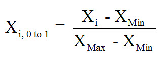
To normalize data, all data values will take on a value of 0 to 1. Since some models collapse at the value of zero, sometimes an arbitrary range of say 0.1 to 0.9 is chosen instead, but for this post I will assume a unity-based normalization. The following equation is what should be used to implement a unity-based normalization:
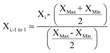
If you desire to have a more centralized set of normalized data, with zero being the central point, then the following equation can be used:
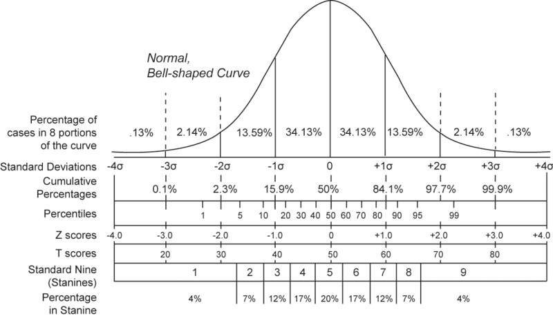
To standardize your data, you will want the data to reflect how many standard deviations from the average that that data lies, with the following normal distribution curve representing the probability of each standard deviation for a normal distribution. The Z-Score is what will be calculated to standardize the data, and it reflects how many standard deviations from the average that the data point falls.
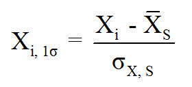
To determine the Z-Score of each data point, the following equation should be used:
Normalized and Standardized can be used to remove their scale from the models. However, standardizing is the preferred method because it produces meaningful information about each data point, and where it falls within its normal distribution, plus provides a crude indicator of outliers.
-
Data Mining Proprocessing in Python
Data mining is a complex process that aims to discover patterns in large data sets. Data Mining some main steps:
-
Collect data: based on the needs
-
Pre-Processing: try to understand the data, denoise and do some dimentation reduction and select the proper predictors, etc
-
Feeding data mining
-
Post-Processing: interpret and evaluate the models
Loading datasets in Python
import pandas as pd
csv_path = 'python_code/data/Heart.csv'
rawdata = pd.read_csv(csv_path)
excel_path = 'python_code/data/energy_efficiency.xlsx'
raw_data2 = pd.read_excel(excel_path)
Understand data with statistics
print "data summary"
print rawdata.describe()
Then you will get
	                 id        year       stint           g          ab
	count    100.000000   100.00000  100.000000  100.000000  100.000000
	mean   89352.660000  2006.92000    1.130000   52.380000  136.540000
	std      218.910859     0.27266    0.337998   48.031299  181.936853
	min    88641.000000  2006.00000    1.000000    1.000000    0.000000
	25%    89353.500000  2007.00000    1.000000    9.500000    2.000000
	50%    89399.000000  2007.00000    1.000000   33.000000   40.500000
	75%    89465.250000  2007.00000    1.000000   83.250000  243.750000
	max    89534.000000  2007.00000    2.000000  155.000000  586.000000
Get the size of the data
nrow, ncol = rawdata.shape
print nrow, ncol
Check the data format
print rawdata.dtypesThen you will get
	id          int64
	player     object
	year        int64
	stint       int64
	team       object
	lg         object
	g           int64
	ab          int64
Get correlation matrix and covariance matrix
# correlation matrix
print "\n correlation Matrix"
print rawdata.corr()
# covariance Matrix
print "\n covariance Matrix"
print rawdata.corr()
Understand data with visualization
from scipy import stats
import seaborn as sns
sns.corrplot(rawdata)
plt.show()

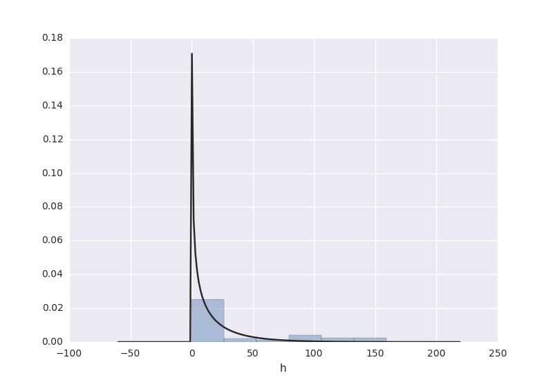
# plot a distribution of observations
attr = rawdata['h']
sns.distplot(attr, kde=False, fit=stats.gamma)
plt.show()

# two subplots, histogram
plt.figure(1)
plt.title("Histogram of stint")
plt.subplot(211) # 2 rows, 1 col
plt.subplot(212) # 2 rows, 1 col
sns.distplot(attr, kde=False, fit=stats.gamma)
plt.show()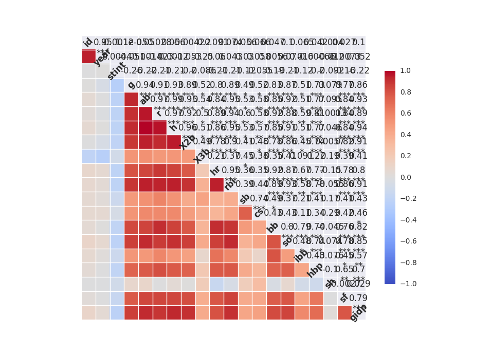
-
-
Machine Learning Intro
In general, a learning problem considers a set of n samples of data and then tries to predict properties (or called features) of unknown data.
We can separate learning problems into a few categories:
supervised learning
data comes with additional attributes that we want to predict:
classification: samples belong to two or more classes and we want to learn from already labeled data how to predict the class of unlabeled data.
regression: if the desired output consists of one or more continuous variables, then the task is called regression.
unsupervised learning
the training data consists of a set of input vectors x without any corresponding target values. The goal in such problems may be to discover groups of similar examples within the data, where it is called clustering, or to determine the distribution of data within the input space, known as density estimation, or to project the data from a high-dimensional space down to two or three dimensions for the purpose of visualization.
What are the top 10 data mining or machine learning algorithms?
One potential answer to this question comes from the Analytics 1305 documentation:
-
Kernel Density Estimation and Non-parametric Bayes Classifier
-
K-Means
-
Kernel Principal Components Analysis
-
Linear Regression
-
Neighbors (Nearest, Farthest, Range, k, Classification)
-
Non-Negative Matrix Factorization
-
Support Vector Machines
-
Dimensionality Reduction
-
Fast Singular Value Decomposition
-
Decision Tree
-
Bootstapped SVM
An awesome Tour of Machine Learning Algorithms was published online by Jason Brownlee in 2013.

-
-
KNN K-Nearest Neighbor Learning and Implementation in Python
- Take a simple example to explain this algorithm:
- How does the KNN algorithm work?
- Implementation in Python
- Example 2
- Explain some parameters in the functions
- When to use the KNN Algorithm
- How do we choose the factor K?
K Nearest Neighbor is one of classification algorithms that are very simple to understand but works incredibly well in practice. Also it is surprisingly versatile and its applications range from vision to proteins to computational geometry to graphs and so on.
When a prediction is required for a unseen data instance, the kNN algorithm will search through the training dataset for the k-most similar instances. The prediction attribute of the most similar instances is summarized and returned as the prediction for the unseen instance.
Take a simple example to explain this algorithm:
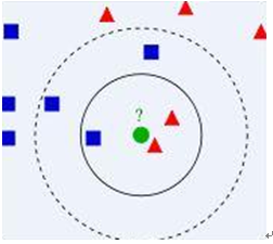
Look at the above image, we have two type data, including blue diamond and red triangle. Assume that we have the green data to determine it belong to which class. How do we do it? We think that only the nearest ones are helpful to find its classification. But how many to determine it? if we choose K=3, then there are 2 red triangles and 1 blue diamond, so we think green one is the same classification of the red one. If we choose K=5, then there are 2 red triangles and 3 blue diamond, so we think green one is the same classification of the blue one.
How does the KNN algorithm work?
Step 1: Calculate the distances between the current node and the nodes in the dataset
Step 2: Sort all the distances
Step 3: Calculate the frequency of the first K nodes in the classes
Step 4: Return the classification with the highest frequence
Implementation in Python
An example in scikit-learn pakage
import numpy as np
import matplotlib.pyplot as plt
from matplotlib.colors import ListedColormap
from sklearn import neighbors, datasets

# import data to play with
iris = datasets.load_iris()
# only two the first two features
X = iris.data[:, :2]
y = iris.target
h = 0.2 # step size in the mesh
n_neighbors = 15

# create the color maps
cmap_light = ListedColormap(['#FFAAAA', '#AAFFAA', '#AAAAFF'])
cmap_bold = ListedColormap(['#FF0000', '#00FF00', '#0000FF'])

for weights in ['uniform', 'distance']:
    # KNN
    clf = neighbors.KNeighborsClassifier(n_neighbors, weights=weights)
    clf.fit(X, y)

    # plot the decision boundary
    x_min, x_max = X[:, 0].min() - 1, X[:, 0].max() + 1
    y_min, y_max = X[:, 1].min() - 1, X[:, 1].max() + 1
    xx, yy = np.meshgrid(np.arange(x_min, x_max, h),
                         np.arange(y_min, y_max, h))
    Z = clf.predict(np.c_[xx.ravel(), yy.ravel()])
    Z = Z.reshape(xx.shape)
    plt.figure()
    plt.pcolormesh(xx, yy, Z, cmap = cmap_light)
    plt.scatter(X[:, 0], X[:, 1], c=y, cmap=cmap_bold)
    plt.xlim(xx.min(), xx.max())
    plt.ylim(yy.min(), yy.max())
    plt.title("3-Class classification (k = %i, weights = '%s')"
              % (n_neighbors, weights))

plt.show()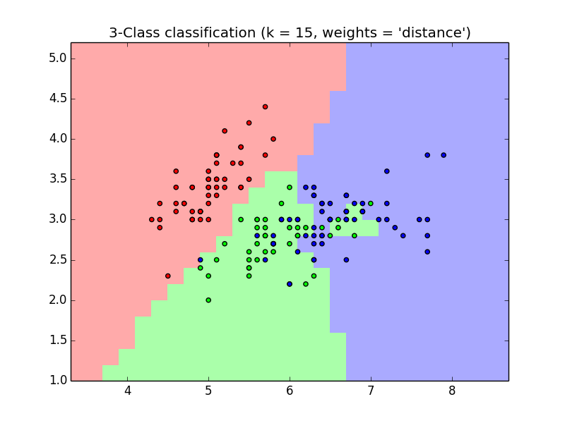
Example 2
import numpy as np
from sklearn import neighbors

knn = neighbors.KNeighborsClassifier()
data = np.array([[3,104],[2,100],[1,81],[101,10],[99,5],[98,2]])
labels = np.array([1,1,1,2,2,2])
knn.fit(data, labels)
knn.predict([18,90])
Explain some parameters in the functions
class sklearn.neighbors.KNeighborsClassifier(n_neighbors=5, weights=’uniform’, algorithm=’auto’, leaf_size=30, p=2, metric=’minkowski’, metric_params=None, n_jobs=1, **kwargs)[source].
n_neighbors: k, means the number of neighbors, default = 5.
weights : str or callable, optional (default = ‘uniform’). ‘uniform’ means all points in each neighborhood are weighted equally. ‘distance’ means that weight points by the inverse of their distance. [callable] : a user-defined function which accepts an array of distances, and returns an array of the same shape containing the weights.
algorithm: ‘auto’, ‘ball_tree’, ‘kd_tree’, ‘brute’.
leaf_size: Leaf size passed to BallTree or KDTree. This can affect the speed of the construction and query, as well as the memory required to store the tree. The optimal value depends on the nature of the problem.
metric: the distance metric to use for the tree.
p: Power parameter for the Minkowski metric.
metric_params: Additional keyword arguments for the metric function.
n_jobs: The number of parallel jobs to run for neighbors search.
When to use the KNN Algorithm
KNN can be used for both classification and regression predictive problems. There are 3 import aspects:
-
Ease to interpret output
-
Calculation time
-
Predictive Power. Graph based KNN is used in protein interaction prediction.
How do we choose the factor K?
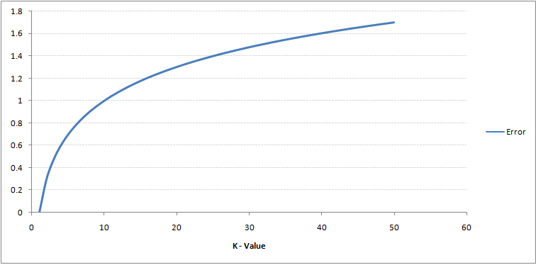
As you can see, the error rate at K=1 is always zero for the training sample. This is because the closest point to any training data point is itself.Hence the prediction is always accurate with K=1. If validation error curve would have been similar, our choice of K would have been 1. Following is the validation error curve with varying value of K:
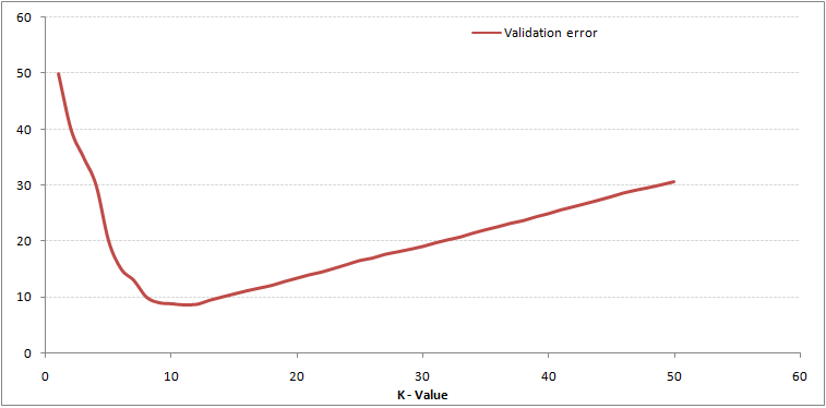
This makes the story more clear. At K=1, we were overfitting the boundaries. Hence, error rate initially decreases and reaches a minima. After the minima point, it then increase with increasing K. To get the optimal value of K, you can segregate the training and validation from the initial dataset. Now plot the validation error curve to get the optimal value of K. This value of K should be used for all predictions.
-
Which is better for data analysis R or Python
This article is from Quora
The answer is from Vik Paruchuri
Python has come up a long way in data analysis with its Scipy, Numpy and Pandas platforms. Is R still a better data analysis language than Python? Has anyone else used Python with Pandas to a large extent in data analysis projects?
For most data analysis projects, your goal is going to be to create the highest quality analysis in the least amount of time.
If you understand the underlying concepts behind what you’re doing, then you can use either language to perform your analysis.
For example, if you understand the principles of natural language processing, data cleaning, and machine learning, you can implement an automated text summarizer in R or Python.
As this blog post shows, the code in R and Python isn’t even that different for most tasks. At Dataquest, we teach data analysis and data science using Python because it’s better for beginners, but we focus on teaching concepts for this reason.
As time goes on, data analysis in R and Python is becoming more similar as great packages like pandas, rvest, and ggplot bring concepts from one language into the other.
Given that, for most cases, I would use whatever language you’re most familiar with. Here are some main points of differentiation between the languages to be aware of, though:
R has a much bigger library of statistical packages
If you’re doing specialized statistical work, R packages cover more techniques. You can find R packages for a wide variety of statistical tasks using the CRAN task view. R packages cover everything from Psychometrics to Genetics to Finance. Although Python, through SciPy and packages like statsmodels, covers the most common techniques, R is far ahead.
Python is better for building analytics tools
R and Python are equally good if you want to find outliers in a dataset, but if you want to create a web service to enable other people to upload datasets and find outliers, Python is better. Python is a general purpose programming language, which means that people have built modules to create websites, interact with a variety of databases, and manage users.
In general, if you want to build a tool or service that uses data analysis, Python is a better choice.
R builds in data analysis functionality by default, whereas Python relies on packages
Because Python is a general purpose language, most data analysis functionality is available through packages like NumPy and pandas. However, R was built with statistics and data analysis in mind, so many tools that have been added to Python through packages are built into base R.
Python is better for deep learning
Through packages like Lasagne, caffe, keras, and tensorflow, creating deep neural networks is straightforward in Python. Although some of these, like tensorflow, are being ported to R, support is still far better in Python.
Python relies on a few main packages, whereas R has hundreds
In Python, sklearn is the “primary” machine learning package, and pandas is the “primary” data analysis package. This makes it easy to know how to accomplish a task, but also means that a lot of specialized techniques aren’t possible.
R, on the other hand, has hundreds of packages and ways to accomplish things. Although there’s generally an accepted way to accomplish things, the lines between base R, packages, and the tidyverse can be fuzzy for inexperienced folks.
R is better for data visualization
Packages like ggplot2 make plotting easier and more customizable in R than in Python. Python is catching up, particularly in the area of interactive plots with packages like Bokeh, but has a way to go.
The bottom line
Performing data analysis tasks in either language is more similar than you might expect. As long as you understand the underlying concepts, pick the language that you’re most familiar with.
R has an edge in statistics and visualization, whereas Python has an advantage in machine learning and building tools.
If you’re new to data analysis, I’d advise learning Python, because it’s more straightforward and more versatile, but I’d also advise focusing on the concepts and quality of the analysis over language. At Dataquest, we teach data science by focusing on the concepts and helping you build projects and add value.
I personally like where tools like Jupyter Notebook and Beaker Notebook are headed in terms of letting you use either language, sometimes in the same analysis.
This article is from Quora