Welcome to Shanshan Blog!

• Python Cheatsheet: Basic

  2017-02-11

  Python

  Python
  • Name Rule
  • future
  • Define function doc
  • Check, Get, Set attribute, inheritance in Class
  • Check global variables
  • Get Function / Class name
  • Diamond Problem
  • Smart List
  • Transfer two list into tuple list
    • Smart Dictionary
    • for else
    • try else
    • lambda function
    • Option arguments

  Name Rule

  # for class
  MyClass
  # for function, module, package, variables
  var_separate
  # for public
  var
  # for private
  __var
  # for internal use
  _var
  # for protect
  _var_
  # convention to avoid conflict keyword
  var_
  # "magic" method or attributes
  __var__
  

  future

  # backport python3 print_function in python2
  from __future__ import print_function
  print "hello world" # errors
  
  # backport python3 unicode_literals in python2
  from __future__ import unicode_literals
  print type("Guido")
  
  # Changing the Division Operator
  from __future__ import division
  print 1/2	#float
  print 1//2 #int
  

  Define function doc

  def Example():
  	""" This is an example function """
  	print "example func"
  
  print Example.__doc__
  # or
  help(Example)
  

  Check, Get, Set attribute, inheritance in Class

  class Example(object):
  	def __init__(self):
  		self.name = "ex"
     	def printex(self):
       	print "This is an example"
  ex = Example()
  print hasattr(ex, "name")
  print getattr(ex,'name')
  setattr(ex, name','example')
  print issubclass(Example, object)
  

  Check global variables

  print globals()
  

  Get Function / Class name

  print ex.__class__.__name__
  

  Diamond Problem

  # The problem of multiple inheritance in searching a method
  def foo_a(self):
  	print("This is ClsA")
  def foo_b(self):
  	print("This is ClsB")
  def foo_c(self):
  	print("This is ClsC")	
  
  class Type(type):
  	def __repr__(cls):
  		return cls.__name__
  
  ClsA = Type("ClsA", (object,), {'foo': foo_a})
  ClsB = Type("ClsB", (ClsA,), {'foo': foo_b})
  ClsC = Type("ClsC", (ClsA,), {'foo': foo_c})
  ClsD = Type("ClsD", (ClsB, ClsC), {})
  ClsD.mro()
  ClsD().foo()				
  

  Smart List

  a = [1, 2, 3, 4, 5]
  print a[0]
  print a[:-1]
  print a[0:-1:2]
  # copy
  ex = [0] * 10
  # extend
  ex = [1, 2, 3] + ['a', 'b']
  # get index and item in the loop
  for idx, item in enumerate(a):
  	print (idx, item),
  

  Transfer two list into tuple list

  zip(a, a)
  # with filter
  [x for x in a if x>1]
  # get distinct val
  list(set(a))
  # reverse a list
  b = a[::-1]
  

  Smart Dictionary

  a = {"1":1, "2":2, "3":3}
  b = {"2":2, "3":3, "4":4}
  print a.keys()
  print a.itemes()
  # find same key between two dictionary
  [_ for _ in a.keys() if _ in b.keys()
  # another way
  c = set(a).intersection(set(b))
  # update dictionary
  a.update(b)
  

  for else

  for _ in range(5):
  	print _,
  else:
  	print "\n no breaks"
  

  try else

  try:
  	print "No exception"
  except:
  	pass
  else:
  	print "No exception occurred"
  

  lambda function

  fn = lambda x: x**2
  

  Option arguments

  def example(a, b=None, *args, **kwargs):
  	print a, b
  	print args
  	print kwargs
  example(1, "var", 2, 3, word="hello")
  

  Read All

  ---

• 500 Lines or Less: Introduction 翻译

  2017-02-10

  Translation

  Python  Translation
  • 介绍
  • Contributing

  这是开源应用程序架构系列中的第四卷，“开源应用”不出现在任何标题中。

  介绍

  该系列系列的前三卷是关于大程序必须解决的大问题。对于一个工程师的早期职业来说，理解和构建比几千多行代码的程序可能是一个挑战，因此，虽然大问题有趣但也具有极具挑战。

  500 Lines or Less 专注于程序员构建新的事物中的一小部分的设计决策。本书中阅读的程序都是从头开始编写的（但有一些程序受到作者过去编写过的大项目的启发）。

  在阅读每一章之前，我们建议你先考虑要如何解决这个问题。你认为作者会认为什么设计考量或约束重要？哪些抽象你期望看到？你认为问题应该如何分解？阅读时尝试找出是什么让你感到惊讶。我们希望你用这样的方式学习，而不是通过从头到尾的阅读每一章来学习。

  为编写一个有用的程序，不到500行的源代码中本身就是一个具有挑战性的工作。还要将之用于教学目的打印在书本上就更是一项艰巨的任务。因此，编辑们将其放到书中时偶尔保留某些源格式。每个章节的源代码在它的项目文件夹的代码子目录中。

  我们希望本书作者们的经验可以帮助你在自己的编程实践中走出你的舒适区。

  Contributing

  如果你想提交相关错误或者翻译内容为其他语言，请打开链接

  Github

  Read All

  ---

• Leetcode (53, 91, 97, 152) Dynamic Programming

  2017-02-09

  Leetcode

  Leetcode  DP
  • Leetcode 53. Maximum Subarray
  • Leetcode 91. Decode Ways
  • Leetcode 97. Interleaving String
  • Leetcode 152. Maximum Product Subarray Add to List

  Dynamic Programming in Leetcode

  Leetcode 53. Maximum Subarray

  Leetcode 53. Maximum Subarray

  Find the contiguous subarray within an array (containing at least one number) which has the largest sum.

  For example, given the array [-2,1,-3,4,-1,2,1,-5,4], the contiguous subarray [4,-1,2,1] has the largest sum = 6.

  Idea: The formula should should be sum[i] = max{A[i], A[i] + sum[i+1]}

  class Solution {
  public:
      int maxSubArray(vector<int>& nums) {
          const int n = nums.size();
          int res[n] = {0};
          res[0] = nums[0];   
          int maxs = nums[0];
          for (int i=1; i<n; i++) 
              res[i] = max(nums[i], res[i-1]+nums[i]);
          for (int i=1; i<n; i++) 
              maxs = max(maxs, res[i]);
          return maxs;
      }
  };
  

  Leetcode 91. Decode Ways

  Leetcode 91. Decode Ways

  A message containing letters from A-Z is being encoded to numbers using the following mapping:

  'A' -> 1 'B' -> 2 ... 'Z' -> 26

  Given an encoded message containing digits, determine the total number of ways to decode it.

  For example,

  Given encoded message “12”, it could be decoded as “AB” (1 2) or “L” (12).

  The number of ways decoding “12” is 2.

  idea:

  动态规划，令dp[i]表示字符串的前i个字符的可能的编码方式的数量。那么递推公式如下：

  如果当前数字为0，则前面数字必为1或者2，否则无法进行编码转换，此时的数字0只能和前面的1或者2连在一起进行编码，因此dp[i] = dp[i-2]； 如果前面数字为1或者前面数字为2且当前数字在1~6之间，说明都可以进行2种编码（分开或者和在一起），因此dp[i] = dp[i-1] + dp[i-2]； 其他情况，当前数字必须单独进行编码转换，因此dp[i] = dp[i-1]。

  class Solution {
  public:
      int numDecodings(string s) {
          const int n = s.size();
          if (n==0 || s[0]=='0')   return 0;
          vector<int>dp(n+1, 0);
          dp[0] = 1;dp[1] = 1;
          for (int i=2; i<=n; i++) {
              if (s[i-1]!='0')  dp[i] = dp[i-1];
              if (s[i-2]=='1'|| (s[i-2]=='2' && s[i-1]>'0' && s[i-1]<'7'))
                  dp[i] += dp[i-2];
              if (s[i-1]=='0' &&(s[i-2]=='1'||s[i-2]=='2'))
                  dp[i] = dp[i-2];
          }
          return dp[n];
      }
  };
  

  Leetcode 97. Interleaving String

  Leetcode 97. Interleaving String

  Given s1, s2, s3, find whether s3 is formed by the interleaving of s1 and s2.

  For example,

  Given:

  s1 = “aabcc”,

  s2 = “dbbca”,

  When s3 = “aadbbcbcac”, return true.

  When s3 = “aadbbbaccc”, return false.

  The idea is from blog

  s1, s2只有两个字符串，因此可以展平为一个二维地图，判断是否能从左上角走到右下角。

  当s1到达第i个元素，s2到达第j个元素:

  地图上往右一步就是s2[j-1]匹配s3[i+j-1]。

  地图上往下一步就是s1[i-1]匹配s3[i+j-1]。

  示例：s1=”aa”,s2=”ab”,s3=”aaba”。标1的为可行。最终返回右下角。

  ` 0 a b

  0 1 1 0

  a 1 1 1

  a 1 0 1 `

  class Solution {
  public:
      bool isInterleave(string s1, string s2, string s3) {
          const int n = s1.size();
          const int m = s2.size();
          const int p = s3.size();
          if (n+m != p)   return false;
          vector<vector<bool>> res(n+1, vector<bool>(m+1, false));
          for (int i=0; i<n+1; i++)
              for (int j=0; j<m+1; j++) {
                  if (i==0 && j==0)   res[i][j]=true;
                  else if (i==0)   res[i][j] = res[i][j-1] & (s2[j-1]==s3[j-1]);
                  else if (j==0)  res[i][j] = res[i-1][j] & (s1[i-1]==s3[i-1]);
                  else    res[i][j] = (res[i-1][j] & (s1[i-1]==s3[i+j-1])) || (res[i][j-1] & (s2[j-1]==s3[i+j-1]));
              } 
          return res[n][m];
      }
  };
  

  Leetcode 152. Maximum Product Subarray Add to List

  Leetcode 152. Maximum Product Subarray Add to List

  Find the contiguous subarray within an array (containing at least one number) which has the largest product.

  For example, given the array [2,3,-2,4], the contiguous subarray [2,3] has the largest product = 6.

  class Solution {
  public:
      int maxProduct(vector<int>& nums) {
          int maxP = 1, minP = 1, res = INT_MIN;
          for (int num: nums) {
              int temp = maxP;
              maxP = max(max(maxP*num, minP*num), num);
              minP = min(min(minP*num, temp*num), num);
              res = max(res, maxP);
          }
          return res;
      }
  };
  

  Read All

  ---

• Hidden Markov Model Example in Python

  2017-02-08

  DataMining

  DataMining
  • Codes

  Codes

  # -*- coding:utf-8 -*-
  from hmmlearn.hmm import GaussianHMM
  import pandas as pd
  import numpy as np
  import matplotlib.pylab as plt
  
  store_path = r"D:\Users\FUSHANSHAN863\Desktop\stock\data\stock.h5"
  store = pd.HDFStore(store_path)
  data = store['data_stock_raw_base']
  store.close()
  data.index = data['data_date']
  # 每日最高最低价格的对数差值
  logDel = np.log(np.array(data['thigh'])) - np.log(np.array(data['tlow']))
  # 每5日的指数对数收益差
  close = data['tclose']
  logRet_1 = np.array(np.diff(np.log(close)))[4:]
  logRet_5 = np.log(np.array(close[5:])) - np.log(np.array(close[:-5]))
  # 每5日的指数成交量的对数差
  volume = data['vaturnover']
  logVol_5 = np.log(np.array(volume[5:])) - np.log(np.array(volume[:-5]))
  
  # 三个特征合成
  feature_select = np.column_stack([logDel[5:],logRet_5,logVol_5])
  
  # HMM model
  model = GaussianHMM(n_components=6, covariance_type="full", n_iter=2000).fit(feature_select)
  hidden_stats = model.predict(feature_select)
  Date = pd.to_datetime(data.index[5:])
  
  plt.figure(figsize=(25, 18))
  for i in range(model.n_components):
      pos = (hidden_stats==i)
      plt.plot_date(Date[pos],close[pos],'o',label='hidden state %d'%i,lw=2)
      plt.legend(loc="left")
  
  plt.show()
  
  
  # 为了测试隐藏状态分别表示什么，假设进行买入操作
  res = pd.DataFrame({'Date':Date,'logRet_1':logRet_1,'state':hidden_stats}).set_index('Date')
  plt.figure(figsize=(25, 18))
  for i in range(model.n_components):
      pos = (hidden_stats==i)
      pos = np.append(0,pos[:-1])#第二天进行买入操作
      df = res.logRet_1
      res['state_ret%s'%i] = df.multiply(pos)
      plt.plot_date(Date,np.exp(res['state_ret%s'%i].cumsum()),'-',label='hidden state %d'%i)
      plt.legend(loc="left")
  
  plt.show()
  
  
  # 假设买入和卖空
  buy = (hidden_stats == 0) + (hidden_stats == 5)
  
  buy = np.append(0,buy[:-1])
  sell = (hidden_stats == 1) + (hidden_stats == 3) \
          + (hidden_stats == 4) + (hidden_stats == 2)
  sell = np.append(0,sell[:-1])
  res['backtest_return'] = res.logRet_1.multiply(buy,axis = 0) \
                              - res.logRet_1.multiply(sell,axis = 0)
  plt.figure(figsize = (15,8))
  plt.plot_date(Date,np.exp(res['backtest_return'].cumsum()),'-',label='backtest result')
  plt.legend()
  plt.grid(1)
  plt.show()
  

  Read All

  ---

• Hidden Markov Model

  2017-02-07

  DataMining

  DataMining
  • Markov Model
  • Hidden Markov Models (HMM)
  • Forward Algorithm
  • Backward Algorithm
  • Viterbi Algorithm

  Markov Model

  In probability theory, a Markov model is a stochastic model used to model randomly changing systems where it is assumed that future states depend only on the current state not on the events that occurred before it (that is, it assumes the Markov property). Generally, this assumption enables reasoning and computation with the model that would otherwise be intractable.

  Hidden Markov Models (HMM)

  A hidden Markov model (HMM) is a statistical Markov model in which the system being modeled is assumed to be a Markov process with unobserved (hidden) states. An HMM can be presented as the simplest dynamic Bayesian network.

  

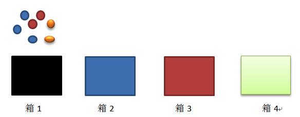
  As we can see, there are 4 boxes, there are balls with 3 different color (blue, red, orange). The staff takes 5 balls from the boxes: red blue blue orange red. It is HMM Process.

  There are 5 components in HMM:

  a. The number of states (4 boxes)

  b. The number of observations (3 colors)

  c. Probability of transition from state ‘i’ to state ‘j’, A= {aij} (the probability of transfering ith box to jth box)

  d. Emission parameter for an observation associated with state i, B={bi(k)} (kth colors ball in ith box)

  e. Initial State π = {πj}. (the probability of the jth box in the first time)

  HMMs commonly solved problems are:

  a. Matching the most likely system to a sequence of observations -evaluation, solved using the forward algorithm;

  b. determining the hidden sequence most likely to have generated a sequence of observations - decoding, solved using the Viterbi algorithm;

  c. determining the model parameters most likely to have generated a sequence of observations - learning, solved using the forward-backward algorithm.

  Forward Algorithm

  Given observations O_1,O_2…O_T, to calculate the si, status in time t

  

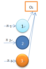
  So

  

  

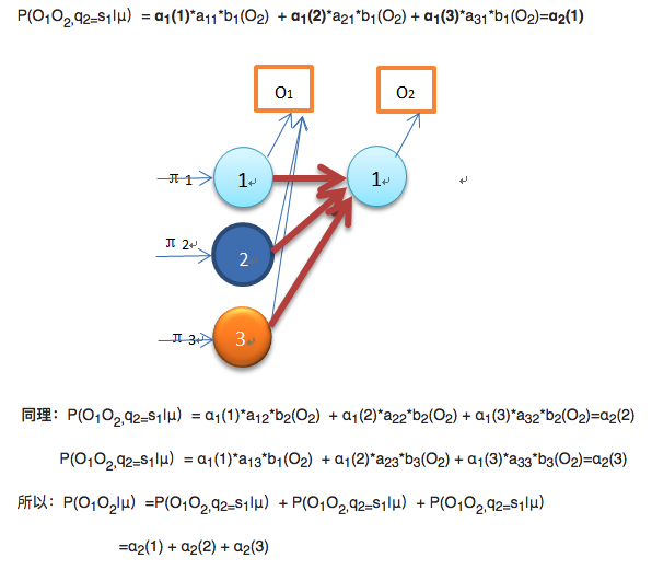
  Time complexity: T*O(N^2)=O(N^2T)

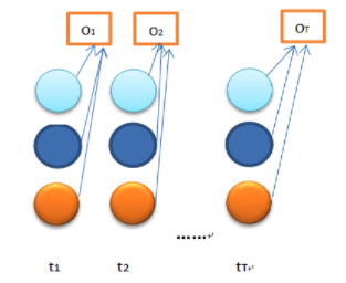
  Backward Algorithm

  Given si, status in time t, calculate the probability of O_t+1, O_t+2…O_T

  

  

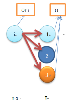
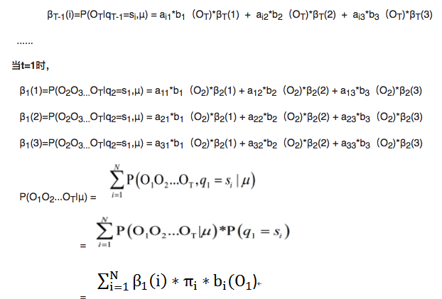
  Time complexity: T*O(N^2)=O(N^2T)

  Viterbi Algorithm

  Determining the hidden sequence most likely to have generated a sequence of observations

  

  The most probable sequence of hidden states is that combination that maximises. This approach is viable, but to find the most probable sequence by exhaustively calculating each combination is computationally expensive.

  Reducing complexity using recursion

  We will consider recursively finding the most probable sequence of hidden states given an observation sequence and a HMM. We will first define the partial probability δ, which is the probability of reaching a particular intermediate state in the trellis. We then show how these partial probabilities are calculated at t=1 and at t=n (> 1).

  a. Partial probabilities (δ’s) and partial best paths

  We will call these paths partial best paths. Each of these partial best paths has an associated probability, the partial probability or δ. Unlike the partial probabilities in the forward algorithm, δis the probability of the one (most probable) path to the state.

  Thus (i,t) is the maximum probability of all sequences ending at state i at time t, and the partial best path is the sequence which achieves this maximal probability. Such a probability (and partial path) exists for each possible value of i and t.

  b. Calculating δ’s at time t = 1

  We calculate the partial probabilities as the most probable route to our current position (given particular knowledge such as observation and probabilities of the previous state). When t = 1 the most probable path to a state does not sensibly exist; however we use the probability of being in that state given t = 1 and the observable state k1 ; i.e.

  

  c. Calculating ‘s at time t ( > 1 )

  We consider calculating the most probable path to the state X at time t; this path to X will have to pass through one of the states A, B or C at time (t-1).

  Therefore the most probable path to X will be one of

  (sequence of states), . . ., A, X

  (sequence of states), . . ., B, X

  (sequence of states), . . ., C, X

  We want to find the path ending AX, BX or CX which has the maximum probability.

  Here, we are assuming knowledge of the previous state, using the transition probabilites and multiplying by the appropriate observation probability. We then select the maximum such.

  

  d. Back pointers, φ’s

  Recall that to calculate the partial probability, δat time t we only need the δ’s for time t-1. Having calculated this partial probability, it is thus possible to record which preceding state was the one to generate δ(i,t) - that is, in what state the system must have been at time t-1 if it is to arrive optimally at state i at time t. This recording (remembering) is done by holding for each state a back pointer which points to the predecessor that optimally provokes the current state.

  Read All

  ---

• Python Cheatsheet: Uniocde

  2017-02-06

  Python

  Python
  • unicode code point to byte
  • byte to unicode code point
  • Get unicode code point

  unicode code point to byte

  s = u'Café'
  print type(s.encode('utf-8'))
  

  byte to unicode code point

  s = bytes('Café', encoding = 'utf-8')
  print s.decode('tuf-8')
  

  Get unicode code point

  for _c in s:print ('U+%04x' % ord(_c))
  # python2 str is equivalent to byte string
  # python3 str is equivalent to unicode string
  

  Read All

  ---