Christian Muise博士是麻省理工学院CSAIL的MERS集团研究员。他对AI,数据驱动项目,绘图,图形理论和数据可视化以及凯尔特音乐,雕刻,足球和咖啡等各种主题都很感兴趣。
流程调度程序
流程车间调度是运营研究中最具挑战性和研究性最强的问题之一。像许多具有挑战性的优化问题一样,找到实际问题的最佳解决方案是不可能的。在本章中,我们考虑使用本地搜索的技术实现流程车间调度结算。本地搜索可以让我们找到一个“不错的”解决方案,找不到最好的解决方案。在给定的时间内尝试找到新的解决方案,并通过返回找到的最佳解决方案来结束程序。
局部搜索背后的思想是通过考虑类似的解决方案来改进现有的解决方案。求解器使用各种策略(1)尝试找到类似的解决方案,(2)选择有可能的探索的解决方案。实现是用Python编写的,没有外部要求。通过利用一些Python不太知名的功能,解决者在解决过程中动态地改变其搜索策略,基于哪些策略运行良好。
首先,我们为流程车间调度问题和局部索技术提供一些背景资料。然后,我们将详细介绍一般的求解器代码以及我们使用的各种启发式和邻域选择策略。接下来,我们考虑解算器用于将所有内容结合在一起的动态策略选择。最后,我们总结一下该项目以及实施过程中获得的经验教训。
背景
流程调度
流程车间调度问题是一个优化问题,其中我们必须确定作业中各种任务的处理时间,以便安排任务以最小化完成作业所需的总时间。例如,一个汽车制造商有一个装配线,其中汽车的每个部分依次在不同的机器上完成。不同的订单可能有自定义的要求,完成制作整体的任务,例如,从一个车到另一个车。在我们的例子中,每辆车都是一项新工作,汽车的每一部分都被称为任务。每个工作都要完成相同的任务顺序。
流程车间调度的目标是最小化处理从每个工作到完成的所有任务所需的总时间。 (通常,这个总时间被称为制造时间)。这个问题有很多应用,但最重要的是优化生产设备。
每个流程车间问题由n个机器和m个作业组成。在我们的汽车示例中,将有n个车站在车上和m车上工作。每个作业都由完整的n任务组成,我们可以假定作业的i任务必须使用机器i,并且需要预定量的处理时间:p(j,i)是作业j的i任务的处理时间。此外,任何给定作业的任务顺序应遵循机器顺序;对于给定的作业,任务i必须在任务i+1开始之前完成。在我们的汽车示例中,我们不想在框架组装之前开始绘画汽车。最后的限制是在机器上不能同时处理两个任务。
因为作业中的任务的顺序是预先确定的,所以可以将流程车间调度问题的解决方案表示为作业的排列。每个机器处理的作业顺序是相同的,并且给定排列,作业j中的机器i的任务计划是以下两种可能性中的最新的:
-
在作业
j-1(即同一机器上的最新任务)中完成机器i的任务,或 -
在作业
j(即同一作业中最近的任务)中完成机器i-1的任务,
因为我们选择这两个值的最大值,所以将创建任一机器i或作业j的空闲时间。正是这个空闲时间,我们最终希望最小化,因为它会使总体制造商的规模更大。
由于问题的简单形式,作业的任何置换都是有效的解决方案,最优解将对应一些置换。因此,我们通过改变作业的排列和测量相应的制作时间来寻找改进的解决方案。在下文中,我们将作业的排列称为候选人。
让我们考虑一个简单的例子,有两个工作和两个机器。第一个工作有任务mathbf{A}和mathbf{B},分别需要1到2分钟才能完成。第二个任务有任务mathbf{C}和`mathbf{D},需要2和1分钟才能完成相应的
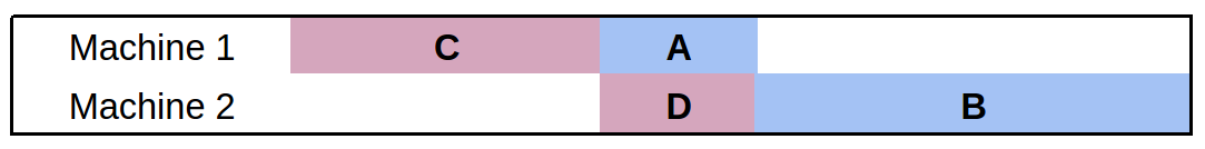
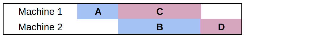
请注意,之前没有多余的空间给任务。良好的排列指导原则是尽可能减少任何机器的运行时间,而无需处理任务。
局部搜索
当最佳解决方案太难计算时,局部搜索是解决优化问题的策略。直观地,它从一个看起来不错的解决方案转向另一种更好的解决方案。我们将所有可能的解决方案都考虑在下一个点之上,而不是将所有可能的解决方案都考虑在内,我们定义了所谓的邻域:被认为与当前解决方案类似的一组解决方案。因为作业的任何排列是一个有效的解决方案,我们可以查看任何将作业当作局部搜索过程进行洗牌的机制。
要使用局部搜索之前,我们必须回答几个问题:
-
如何开始?
-
基于给出的解决方案,我们应该考虑什么邻近的解决方案?
-
基于候选邻居的集合,考虑哪一个作为下一个?
以下三个部分依次讨论这些问题。
一般解决方案
在本节中,我们提供了流程车间调度程序的一般框架。首先,我们有必要的Python导入和解算器的设置:
import sys, os, time, random

from functools import partial
from collections import namedtuple
from itertools import product

import neighbourhood as neigh
import heuristics as heur

##############
## Settings ##
##############
TIME_LIMIT = 300.0 # Time (in seconds) to run the solver
TIME_INCREMENT = 13.0 # Time (in seconds) in between heuristic measurements
DEBUG_SWITCH = False # Displays intermediate heuristic info when True
MAX_LNS_NEIGHBOURHOODS = 1000 # Maximum number of neighbours to explore in LNS
有两个设置应该进一步解释下。TIME_INCREMENT设置作动态策略选择,MAX_LNS_NEIGHBOURHOODS设置邻域选择策略。 两者在下面更详细地描述。
这些设置可以作为命令行参数暴露给用户,但在此阶段,我们将输入数据作为参数提供给程序。 输入问题 - 来自Taillard基准集的问题被假定为用于流程车间调度的标准格式。 以下代码用作求解器文件的__main__方法,并根据输入到程序的参数数调用相应的函数:
if __name__ == '__main__':

    if len(sys.argv) == 2:
        data = parse_problem(sys.argv[1], 0)
    elif len(sys.argv) == 3:
        data = parse_problem(sys.argv[1], int(sys.argv[2]))
    else:
        print "\nUsage: python flow.py <Taillard problem file> [<instance number>]\n"
        sys.exit(0)

    (perm, ms) = solve(data)
    print_solution(data, perm)
我们将尽快描述Taillard问题文件的解析。(这些文件可以在线获得)
解决方案期望数据变量是包含每个作业的活动持续时间的整数列表。从初始化一组全局策略开始。 关键是我们使用strat_ *变量来维护每个策略的统计信息。这有助于在解决过程中动态选择策略。
def solve(data):
    """Solves an instance of the flow shop scheduling problem"""

    # We initialize the strategies here to avoid cyclic import issues
    initialize_strategies()
    global STRATEGIES

    # Record the following for each strategy:
    #  improvements: The amount a solution was improved by this strategy
    #  time_spent: The amount of time spent on the strategy
    #  weights: The weights that correspond to how good a strategy is
    #  usage: The number of times we use a strategy
    strat_improvements = {strategy: 0 for strategy in STRATEGIES}
    strat_time_spent = {strategy: 0 for strategy in STRATEGIES}
    strat_weights = {strategy: 1 for strategy in STRATEGIES}
    strat_usage = {strategy: 0 for strategy in STRATEGIES}
流程车间调度问题一个吸引人的特征是每个排列都是一个有效的解决方案,至少有一个最佳的制作时间。幸运的是,这允许我们放弃检查,当从一个排列到另一个排列时,保持可行解决方案的空间下 - 一切都是可行的!
然而,要在排列空间中开始局部搜索,我们必须进行初始置换。为了让事情变得简单,我们会随机抽取工作列表来填补局部搜索:
    # Start with a random permutation of the jobs
    perm = range(len(data))
    random.shuffle(perm)
接下来,我们初始化允许我们跟踪到目前为止发现的最佳排列的变量,以及提供输出的时序信息。
    # Keep track of the best solution
    best_make = makespan(data, perm)
    best_perm = perm
    res = best_make

    # Maintain statistics and timing for the iterations
    iteration = 0
    time_limit = time.time() + TIME_LIMIT
    time_last_switch = time.time()

    time_delta = TIME_LIMIT / 10
    checkpoint = time.time() + time_delta
    percent_complete = 10

    print "\nSolving..."
由于这是局部搜索解决方案,我们只要继续尝试改进解决方案,只要时间没有到。我们提供指示求解器进度的输出,并跟踪我们计算出的迭代次数:
    while time.time() < time_limit:

        if time.time() > checkpoint:
            print " %d %%" % percent_complete
            percent_complete += 10
            checkpoint += time_delta

        iteration += 1
下面我们会描述如何选择策略,但是现在只要知道该策略提供邻域函数和启发式函数就足够了。前者为我们提供了neighbourhood的方法,而后者从该组中选出最佳候选人。从这些函数,我们有一个新的排列(perm)和一个新的makepan结果(res):
        # Heuristically choose the best strategy
        strategy = pick_strategy(STRATEGIES, strat_weights)

        old_val = res
        old_time = time.time()

        # Use the current strategy's heuristic to pick the next permutation from
        # the set of candidates generated by the strategy's neighbourhood
        candidates = strategy.neighbourhood(data, perm)
        perm = strategy.heuristic(data, candidates)
        res = makespan(data, perm)
用于计算makepan的代码非常简单:我们可以通过评估最终作业完成时的排列来计算它。我们将在下面看到compile_solution如何工作,但现在只需知道一个2D数组,并且[-1][-1]中的元素对应于调度中最后一个作业的开始时间:
def makespan(data, perm):
    """Computes the makespan of the provided solution"""
    return compile_solution(data, perm)[-1][-1] + data[perm[-1]][-1]
为了帮助选择策略,我们保留统计数据(1)策略有多大改进了解决方案,(2)策略花了多少时间用于计算信息,以及(3)使用策略的次数。如果我们有更好的解决方案,我们还会更新最佳排列的变量:
        # Record the statistics on how the strategy did
        strat_improvements[strategy] += res - old_val
        strat_time_spent[strategy] += time.time() - old_time
        strat_usage[strategy] += 1

        if res < best_make:
            best_make = res
            best_perm = perm[:]
使用统计数据定期更新战略。为了可读性我们删除了相关的片段,并详细说明下面的代码。 作为最后一步,一旦while循环完成(即达到时间限制),我们输出一些有关求解过程的统计信息,并返回最佳排列顺序及其排序:
    print " %d %%\n" % percent_complete
    print "\nWent through %d iterations." % iteration

    print "\n(usage) Strategy:"
    results = sorted([(strat_weights[STRATEGIES[i]], i)
                      for i in range(len(STRATEGIES))], reverse=True)
    for (w, i) in results:
        print "(%d) \t%s" % (strat_usage[STRATEGIES[i]], STRATEGIES[i].name)

    return (best_perm, best_make)
解析问题
作为解析过程的输入,我们提供可以找到输入的文件名和应该使用的示例编号。 (每个文件包含一些实例。)
def parse_problem(filename, k=1):
    """Parse the kth instance of a Taillard problem file

    The Taillard problem files are a standard benchmark set for the problem
    of flow shop scheduling.

    print "\nParsing..."
通过读取文件并识别分隔每个问题实例的行来开始解析:
    with open(filename, 'r') as f:
        # Identify the string that separates instances
        problem_line = ('/number of jobs, number of machines, initial seed, '
                        'upper bound and lower bound :/')

        # Strip spaces and newline characters from every line
        lines = map(str.strip, f.readlines())
为了更容易地查找正确的实例,我们假设行用’/’字符分隔。根据出现在每个实例顶部的公共字符串来分割文件,并且在第一行的开始处添加一个“/”字符允许下面的字符串处理正常工作。在文件中发现的实例集合中,我们还会检测提供的实例号是否超出范围。
        # We prep the first line for later
        lines[0] = '/' + lines[0]

        # We also know '/' does not appear in the files, so we can use it as
        #  a separator to find the right lines for the kth problem instance
        try:
            lines = '/'.join(lines).split(problem_line)[k].split('/')[2:]
        except IndexError:
            max_instances = len('/'.join(lines).split(problem_line)) - 1
            print "\nError: Instance must be within 1 and %d\n" % max_instances
            sys.exit(0)
我们直接解析数据,将每个任务的处理时间转换为一个整数,并将其存储在列表中。最后,压缩数据来反转行和列,使格式符合上述求解代码的期望值。(数据中的每个项目都应该对应于特定的作业。)
        # Split every line based on spaces and convert each item to an int
        data = [map(int, line.split()) for line in lines]

    # We return the zipped data to rotate the rows and columns, making each
    #  item in data the durations of tasks for a particular job
    return zip(*data)
编译解决方案
流程车间调度问题的解决方案包括每个作业中每个任务的精确时序。因为我们用作业的排列隐含地表示一个解决方案,所以我们引入了compile_solution函数置换转换为精确的时间。作为输入,函数所需要的数据和作业的排列。
该函数通过初始化用于存储每个任务的开始时间的数据结构,然后在排列中包括来自第一个作业的任务。
def compile_solution(data, perm):
    """Compiles a scheduling on the machines given a permutation of jobs"""

    num_machines = len(data[0])

    # Note that using [[]] * m would be incorrect, as it would simply
    #  copy the same list m times (as opposed to creating m distinct lists).
    machine_times = [[] for _ in range(num_machines)]

    # Assign the initial job to the machines
    machine_times[0].append(0)
    for mach in range(1,num_machines):
        # Start the next task in the job when the previous finishes
        machine_times[mach].append(machine_times[mach-1][0] +
                                   data[perm[0]][mach-1])
然后我们为剩余的作业添加所有任务。 一旦上一个作业的第一个任务完成,作业中的第一个任务就启动。 对于剩余的任务,我们尽可能早地安排作业:同一作业中上一个任务的完成时间的最大值以及同一台机器上的上一个任务的完成时间。
    # Assign the remaining jobs
    for i in range(1, len(perm)):

        # The first machine never contains any idle time
        job = perm[i]
        machine_times[0].append(machine_times[0][-1] + data[perm[i-1]][0])

        # For the remaining machines, the start time is the max of when the
        #  previous task in the job completed, or when the current machine
        #  completes the task for the previous job.
        for mach in range(1, num_machines):
            machine_times[mach].append(max(
                machine_times[mach-1][i] + data[perm[i]][mach-1],
                machine_times[mach][i-1] + data[perm[i-1]][mach]))

    return machine_times
打印解决方案
解决过程完成后,程序输出有关解决方案的信息。我们不是为每个工作提供每个任务的精确时间,而是输出以下信息:
-
产生最佳制作工作的排列
-
计算的排列的完成时间
-
每个机器的开始时间,完成时间和空闲时间
-
每个工作的开始时间,完成时间和空闲时间
作业或机器的开始时间对应于作业或机器上第一个任务的开始。类似地,作业或机器的完成时间对应于作业或机器上的最终任务的结束。空闲时间是特定作业或机器的任务之间的松弛量。理想情况下,我们希望减少空闲时间,因为这意味着整个流程的时间也会减少。
已经讨论了编译解决方案的代码(即计算每个任务的开始时间),并输出排列和排序是简单的:
def print_solution(data, perm):
    """Prints statistics on the computed solution"""

    sol = compile_solution(data, perm)

    print "\nPermutation: %s\n" % str([i+1 for i in perm])

    print "Makespan: %d\n" % makespan(data, perm)
接下来,我们使用Python中字符串格式化的功能来打印每个机器和作业的开始,结束和空闲时间表 请注意,作业的空闲时间是从作业开始到完成的时间,减去作业中每个任务的处理时间的总和。我们以类似的方式计算机器的空闲时间。
    row_format ="{:>15}" * 4
    print row_format.format('Machine', 'Start Time', 'Finish Time', 'Idle Time')
    for mach in range(len(data[0])):
        finish_time = sol[mach][-1] + data[perm[-1]][mach]
        idle_time = (finish_time - sol[mach][0]) - sum([job[mach] for job in data])
        print row_format.format(mach+1, sol[mach][0], finish_time, idle_time)

    results = []
    for i in range(len(data)):
        finish_time = sol[-1][i] + data[perm[i]][-1]
        idle_time = (finish_time - sol[0][i]) - sum([time for time in data[perm[i]]])
        results.append((perm[i]+1, sol[0][i], finish_time, idle_time))

    print "\n"
    print row_format.format('Job', 'Start Time', 'Finish Time', 'Idle Time')
    for r in sorted(results):
        print row_format.format(*r)

    print "\n\nNote: Idle time does not include initial or final wait time.\n"
Neighbourhoods
局部搜索背后的想法是从一个解决方案移到邻近的解决方案。We refer to the neighbourhood of a given solution as the other solutions that are local to it. 在本节中,我们详细介绍了四个潜在的社区,每个社区的复杂程度日益增加。
第一个邻域产生给定数量的随机排列。这个neighbourhood甚至不考虑我们最初的解决方案,所以使用了neighbourhood一词。然而,包括搜索中的一些随机性是好的,因为它促进了搜索空间的探索。
def neighbours_random(data, perm, num = 1):
    # Returns <num> random job permutations, including the current one
    candidates = [perm]
    for i in range(num):
        candidate = perm[:]
        random.shuffle(candidate)
        candidates.append(candidate)
    return candidates
对于下一个neighbour,我们考虑在排列中交换两个作业。 通过使用itertools包中的combinations函数,我们可以轻松地遍历每对索引,并创建一个对应于交换位于每个索引的作业的新排列。在某种意义上,neighbour创造了和开始的排列非常相似的排列。
def neighbours_swap(data, perm):
    # Returns the permutations corresponding to swapping every pair of jobs
    candidates = [perm]
    for (i,j) in combinations(range(len(perm)), 2):
        candidate = perm[:]
        candidate[i], candidate[j] = candidate[j], candidate[i]
        candidates.append(candidate)
    return candidates
我们考虑的下一个neighbour使用特定于手头问题的信息。我们找到空闲时间最多的工作,并考虑以各种方式交换。我们收取一个值size,这是我们考虑的工作数量:大多数空闲工作的size。该过程的第一步是计算排列中每个作业的空闲时间:
def neighbours_idle(data, perm, size=4):
    # Returns the permutations of the <size> most idle jobs
    candidates = [perm]

    # Compute the idle time for each job
    sol = flow.compile_solution(data, perm)
    results = []

    for i in range(len(data)):
        finish_time = sol[-1][i] + data[perm[i]][-1]
        idle_time = (finish_time - sol[0][i]) - sum([t for t in data[perm[i]]])
        results.append((idle_time, i))
接下来,计算有最大理想时间的size工作的列表。
    # Take the <size> most idle jobs
    subset = [job_ind for (idle, job_ind) in reversed(sorted(results))][:size]
最后,通过考虑确定的大多数空闲工作的每个排列来构建neighbourhood。为了找到这个排列,我们利用了itertools包中的permutations函数:
    # Enumerate the permutations of the idle jobs
    for ordering in permutations(subset):
        candidate = perm[:]
        for i in range(len(ordering)):
            candidate[subset[i]] = perm[ordering[i]]
        candidates.append(candidate)

    return candidates
我们认为最后的neighbourhood通常被称为大邻域搜索(LNS)。直观地,LNS通过考虑当前排列的小子集来工作,隔离定位工作子集的最佳排列给我们一个LNS neighbourhood的候选者。通过对特定大小的几个(或全部)子集重复此过程,我们可以增加附近的候选人数。 我们限制通过MAX_LNS_NEIGHBOURHOODS参数考虑的数字,因为neighbourhood的数量可以很快增长。 LNS计算的第一步是使用itertools包的combinations函数来计算我们将考虑交换的作业集的随机列表:
def neighbours_LNS(data, perm, size = 2):
    # Returns the Large Neighbourhood Search neighbours
    candidates = [perm]

    # Bound the number of neighbourhoods in case there are too many jobs
    neighbourhoods = list(combinations(range(len(perm)), size))
    random.shuffle(neighbourhoods)
接下来,我们遍历子集,以找到每个作业的最佳排列。我们已经看到了类似的代码,用于遍历大多数空闲作业的所有排列。这里的关键区别在于,我们仅记录子集的最佳排列,因为通过为考虑的作业的每个子集选择一个置换来构建较大的neighbour。
    for subset in neighbourhoods[:flow.MAX_LNS_NEIGHBOURHOODS]:

        # Keep track of the best candidate for each neighbourhood
        best_make = flow.makespan(data, perm)
        best_perm = perm

        # Enumerate every permutation of the selected neighbourhood
        for ordering in permutations(subset):
            candidate = perm[:]
            for i in range(len(ordering)):
                candidate[subset[i]] = perm[ordering[i]]
            res = flow.makespan(data, candidate)
            if res < best_make:
                best_make = res
                best_perm = candidate

        # Record the best candidate as part of the larger neighbourhood
        candidates.append(best_perm)

    return candidates
如果我们要将size参数设置为等于作业数量,那么每个排列都将被考虑并且选择最好的。但实际上,我们需要将子集的大小限制在3或4左右; 任何较大的事情都会导致neighbours_LNS的时间过长。
启发式
启发式从一组提供的候选中返回单个候选排列。 启发式还可以访问问题数据,以评估哪个候选人可能是首选。
我们考虑的第一个启发式是heur_random。该启发式从列表中随机选择一个候选项,而不评估哪一个可能是首选的:
def heur_random(data, candidates):
    # Returns a random candidate choice
    return random.choice(candidates)
下一个启发式的heur_hillclimbing使用另一个极端。它不是随机选择候选人,而是选择具有最佳制作时间的候选人。请注意,列表scores将包含形式(make,perm)的元组,其中make是排列perm创造的价值。 排序这样的列表将列表中开始的最佳制作时间的元组放置; 从这个元组我们返回排列。
def heur_hillclimbing(data, candidates):
    # Returns the best candidate in the list
    scores = [(flow.makespan(data, perm), perm) for perm in candidates]
    return sorted(scores)[0][1]
最后的启发式,heur_random_hillclimbing,结合了上面的随机和爬坡启发式。执行局部搜索时,您可能不一定要选择随机候选人,甚至是最好的候选人。 heur_random_hillclimbing启发式通过选择概率为0.5的最佳候选者返回“不错”的解决方案,然后以概率0.25选择第二最佳候选者,依此类推。while循环在每次迭代时基本上翻转硬币,以查看它是否应该继续增加索引(对列表的大小有限制)。选择的最终索引对应于启发式选择的候选者。
def heur_random_hillclimbing(data, candidates):
    # Returns a candidate with probability proportional to its rank in sorted quality
    scores = [(flow.makespan(data, perm), perm) for perm in candidates]
    i = 0
    while (random.random() < 0.5) and (i < len(scores) - 1):
        i += 1
    return sorted(scores)[i][1]
由于完成时间是我们优化的目标,因此hillclimbing将引导局部搜索找到更好的解决方案。引入随机性使我们能够探索neighbourhood,而不是盲目地寻找更好的解决方案。
动态策略选择
拒不搜索排列的核心是使用特定的启发式和neighbourhood函数从一个解决方案跳转到另一个解决方案。我们如何进行选择呢?实际上,在搜索过程中,它经常有助于切换策略。我们使用的动态策略选择将在启发式和邻域函数的组合之间进行切换,以便尝试并动态地转换为最有效的策略。对于我们来说,策略是启发式和neighbourhood函数(包括其参数值)的特定配置。
首先,我们的代码构建了我们想要解决的策略范围。在策略初始化中,我们使用functools包中的partial函数分配每个邻域的参数。另外,我们构建了启发式函数的列表,最后我们使用产品运算符将每个邻域和启发式函数的组合作为新的策略。
################
## Strategies ##
#################################################
## A strategy is a particular configuration
##  of neighbourhood generator (to compute
##  the next set of candidates) and heuristic
##  computation (to select the best candidate).
##

STRATEGIES = []

# Using a namedtuple is a little cleaner than using dictionaries.
#  E.g., strategy['name'] versus strategy.name
Strategy = namedtuple('Strategy', ['name', 'neighbourhood', 'heuristic'])

def initialize_strategies():

    global STRATEGIES

    # Define the neighbourhoods (and parameters) that we would like to use
    neighbourhoods = [
        ('Random Permutation', partial(neigh.neighbours_random, num=100)),
        ('Swapped Pairs', neigh.neighbours_swap),
        ('Large Neighbourhood Search (2)', partial(neigh.neighbours_LNS, size=2)),
        ('Large Neighbourhood Search (3)', partial(neigh.neighbours_LNS, size=3)),
        ('Idle Neighbourhood (3)', partial(neigh.neighbours_idle, size=3)),
        ('Idle Neighbourhood (4)', partial(neigh.neighbours_idle, size=4)),
        ('Idle Neighbourhood (5)', partial(neigh.neighbours_idle, size=5))
    ]

    # Define the heuristics that we would like to use
    heuristics = [
        ('Hill Climbing', heur.heur_hillclimbing),
        ('Random Selection', heur.heur_random),
        ('Biased Random Selection', heur.heur_random_hillclimbing)
    ]

    # Combine every neighbourhood and heuristic strategy
    for (n, h) in product(neighbourhoods, heuristics):
        STRATEGIES.append(Strategy("%s / %s" % (n[0], h[0]), n[1], h[1]))
一旦定义了策略,我们就不一定要在搜索过程中坚持使用单个选项。相反,我们随机选择任何策略,但是根据策略执行情况对选择进行加权。 我们描述下面的权重,但是对于pick_strategy函数,我们只需要一个策略列表和相应的权重列表(任何数字都可以)。要选择具有给定权重的随机策略,我们在0和所有权重的和之间均匀地选取一个数字。 随后,我们找到最小的索引i,使得小于i的索引的所有权重的总和大于我们选择的随机数。 这种技术,有时被称为轮盘选择,将随机为我们选择一个策略,并把更大的机会给那些更重的策略。
def pick_strategy(strategies, weights):
    # Picks a random strategy based on its weight: roulette wheel selection
    #  Rather than selecting a strategy entirely at random, we bias the
    #  random selection towards strategies that have worked well in the
    #  past (according to the weight value).
    total = sum([weights[strategy] for strategy in strategies])
    pick = random.uniform(0, total)
    count = weights[strategies[0]]

    i = 0
    while pick > count:
        count += weights[strategies[i+1]]
        i += 1

    return strategies[i]
剩下的是描述在寻找解决方案时如何增加权重。这种情况发生在求解器的主while循环中,定期定时(由TIME_INCREMENT变量定义):
        # At regular intervals, switch the weighting on the strategies available.
        #  This way, the search can dynamically shift towards strategies that have
        #  proven more effective recently.
        if time.time() > time_last_switch + TIME_INCREMENT:

            time_last_switch = time.time()
回想一下,strat_improvements存储策略所做的所有改进的总和,而strat_time_spent存储在最后一个时间间隔内给出策略的时间。我们规范了每个策略花费的总时间的改进,以获得每个策略在最后一个时间间隔内执行的进度。因为策略可能没有机会运行,所以我们选择少量的时间作为默认值。
            # Normalize the improvements made by the time it takes to make them
            results = sorted([
                (float(strat_improvements[s]) / max(0.001, strat_time_spent[s]), s)
                for s in STRATEGIES])
现在,我们对每个策略的表现进行排名,我们将k加到最佳策略的权重(假设我们有k个策略),k-1为下一个最佳策略等。每个策略的重量都会增加,列表中最差的策略将只增加1。
            # Boost the weight for the successful strategies
            for i in range(len(STRATEGIES)):
                strat_weights[results[i][1]] += len(STRATEGIES) - i
我们还人为地增加了所有未被使用的策略。这样做是为了让我们不要完全忘记一个策略。虽然一开始就有一个策略可能表现不佳,但后来在搜索中可以证明是非常有用的。
                # Additionally boost the unused strategies to avoid starvation
                if results[i][0] == 0:
                    strat_weights[results[i][1]] += len(STRATEGIES)
最后,我们输出有关策略排名的一些信息(如果设置了DEBUG_SWITCH标志),并且在下一个时间间隔内重置strat_improvements和strat_time_spent变量。
            if DEBUG_SWITCH:
                print "\nComputing another switch..."
                print "Best: %s (%d)" % (results[0][1].name, results[0][0])
                print "Worst: %s (%d)" % (results[-1][1].name, results[-1][0])
                print results
                print sorted([strat_weights[STRATEGIES[i]]
                              for i in range(len(STRATEGIES))])

            strat_improvements = {strategy: 0 for strategy in STRATEGIES}
            strat_time_spent = {strategy: 0 for strategy in STRATEGIES}
讨论
在本章中,我们已经看到可以用相对较少量的代码来实现,以解决流程车间调度的复杂优化问题。找到最佳解决方案可以解决很大的优化问题,如流动车间难度大。在这种情况下,我们可以转向近似技术,如局部搜索来计算一个足够好的解决方案。通过局部搜索,我们可以从一个解决方案转移到另一个解决方案,旨在找到质量好的解决方案。
局部搜索一般可以应用于广泛的问题。我们专注于(1)从一个候选解决方案生成问题的相关解决方案的neighbourhood,以及(2)建立评估和比较解决方案的方法。使用这两个组件,当最佳选项太难计算时,我们可以使用局部搜索范例来找到有价值的解决方案。
我们看到如何在解决过程中动态地选择一种策略来转移,而不是使用任何一种策略来解决问题。这种简单而强大的技术使程序能够混合和匹配部分策略来解决现有问题,这也意味着开发人员不必手工定制策略。