Markov Model
In probability theory, a Markov model is a stochastic model used to model randomly changing systems where it is assumed that future states depend only on the current state not on the events that occurred before it (that is, it assumes the Markov property). Generally, this assumption enables reasoning and computation with the model that would otherwise be intractable.
Hidden Markov Models (HMM)
A hidden Markov model (HMM) is a statistical Markov model in which the system being modeled is assumed to be a Markov process with unobserved (hidden) states. An HMM can be presented as the simplest dynamic Bayesian network.
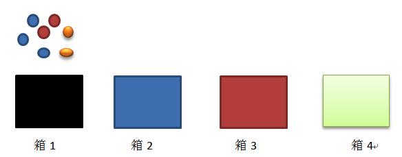
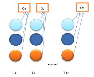
As we can see, there are 4 boxes, there are balls with 3 different color (blue, red, orange). The staff takes 5 balls from the boxes: red blue blue orange red. It is HMM Process.
There are 5 components in HMM:
a. The number of states (4 boxes)
b. The number of observations (3 colors)
c. Probability of transition from state ‘i’ to state ‘j’, A= {aij} (the probability of transfering ith box to jth box)
d. Emission parameter for an observation associated with state i, B={bi(k)} (kth colors ball in ith box)
e. Initial State π = {πj}. (the probability of the jth box in the first time)
HMMs commonly solved problems are:
a. Matching the most likely system to a sequence of observations -evaluation, solved using the forward algorithm;
b. determining the hidden sequence most likely to have generated a sequence of observations - decoding, solved using the Viterbi algorithm;
c. determining the model parameters most likely to have generated a sequence of observations - learning, solved using the forward-backward algorithm.
Forward Algorithm
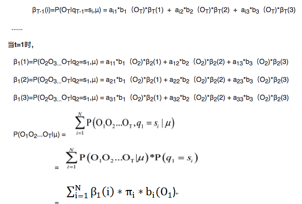
Given observations O_1,O_2…O_T, to calculate the si, status in time t
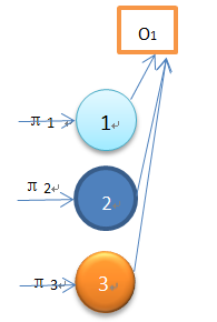
So

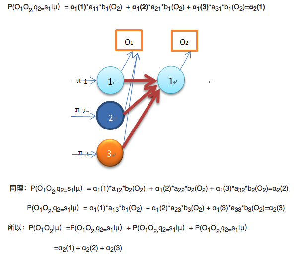
Time complexity: T*O(N^2)=O(N^2T)
Backward Algorithm
Given si, status in time t, calculate the probability of O_t+1, O_t+2…O_T
Time complexity: T*O(N^2)=O(N^2T)
Viterbi Algorithm
Determining the hidden sequence most likely to have generated a sequence of observations
The most probable sequence of hidden states is that combination that maximises. This approach is viable, but to find the most probable sequence by exhaustively calculating each combination is computationally expensive.
Reducing complexity using recursion
We will consider recursively finding the most probable sequence of hidden states given an observation sequence and a HMM. We will first define the partial probability δ, which is the probability of reaching a particular intermediate state in the trellis. We then show how these partial probabilities are calculated at t=1 and at t=n (> 1).
a. Partial probabilities (δ’s) and partial best paths
We will call these paths partial best paths. Each of these partial best paths has an associated probability, the partial probability or δ. Unlike the partial probabilities in the forward algorithm, δis the probability of the one (most probable) path to the state.
Thus (i,t) is the maximum probability of all sequences ending at state i at time t, and the partial best path is the sequence which achieves this maximal probability. Such a probability (and partial path) exists for each possible value of i and t.
b. Calculating δ’s at time t = 1
We calculate the partial probabilities as the most probable route to our current position (given particular knowledge such as observation and probabilities of the previous state). When t = 1 the most probable path to a state does not sensibly exist; however we use the probability of being in that state given t = 1 and the observable state k1 ; i.e.
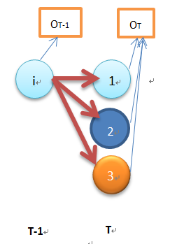
c. Calculating ‘s at time t ( > 1 )
We consider calculating the most probable path to the state X at time t; this path to X will have to pass through one of the states A, B or C at time (t-1).
Therefore the most probable path to X will be one of
(sequence of states), . . ., A, X
(sequence of states), . . ., B, X
(sequence of states), . . ., C, X
We want to find the path ending AX, BX or CX which has the maximum probability.
Here, we are assuming knowledge of the previous state, using the transition probabilites and multiplying by the appropriate observation probability. We then select the maximum such.
d. Back pointers, φ’s
Recall that to calculate the partial probability, δat time t we only need the δ’s for time t-1. Having calculated this partial probability, it is thus possible to record which preceding state was the one to generate δ(i,t) - that is, in what state the system must have been at time t-1 if it is to arrive optimally at state i at time t. This recording (remembering) is done by holding for each state a back pointer which points to the predecessor that optimally provokes the current state.