- prepare data and packages
- Draw data to see the overview
- ADF test for checking the series stable or not
- Make series data Stationary
- Prediction: ARIMA model
- Go back to the origin data
prepare data and packages
Pandas has dedicated libraries for handling TS objects, particularly the datatime64[ns] class which stores time information and allows us to perform some operations really fast. Lets start by firing up the required libraries:
# -*- coding:utf-8 -*-
import pandas as pd
import numpy as np
import matplotlib.pylab as plt
from statsmodels.tsa.stattools import adfuller

from matplotlib.pylab import rcParams
rcParams['figure.figsize'] = 15, 6
from statsmodels.tsa.arima_model import ARIMA
from statsmodels.tsa.seasonal import seasonal_decompose
from statsmodels.tsa.stattools import acf, pacf

# 设置时间格式
dateparse = lambda dates: pd.datetime.strptime(dates, '%Y-%m')
# 读取数据时,见时间设置作为索引
data = pd.read_csv('AirPassengers.csv', index_col='Month',date_parser=dateparse)
ts = data['#Passengers']
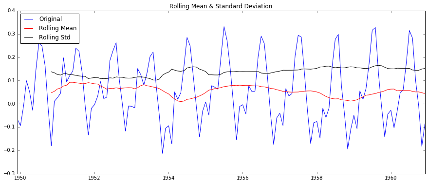
Draw data to see the overview
def draw(timeseries):
    rolmean = pd.rolling_mean(timeseries, window=12)
    rolstd = pd.rolling_std(timeseries, window=12)
    orig = plt.plot(timeseries, color='blue', label='Original')
    mean = plt.plot(rolmean, color='red', label='Rolling Mean')
    std = plt.plot(rolstd, color='black', label='Rolling Std')
    plt.legend(loc='best')
    plt.title('Rolling Mean & Standard Deviation')
    plt.show()

plt.plot(ts)
ADF test for checking the series stable or not
# ADF 检验
def test_stationarity(timeseries):
    # Perform Dickey-Fuller test:
    print 'Results of Dickey-Fuller Test:'
    dftest = adfuller(timeseries, autolag='AIC')
    dfoutput = pd.Series(dftest[0:4], index=['Test Statistic', 'p-value', '#Lags Used', 'Number of Observations Used'])
    for key, value in dftest[4].items():
        dfoutput['Critical Value (%s)' % key] = value
    print dfoutput
The result is:
	Results of Dickey-Fuller Test:
	Test Statistic                   0.815369
	p-value                          0.991880
	#Lags Used                      13.000000
	Number of Observations Used    130.000000
	Critical Value (5%)             -2.884042
	Critical Value (1%)             -3.481682
	Critical Value (10%)            -2.578770
	dtype: float64
Note that the signed values should be compared and not the absolute values.
Make series data Stationary
# method 1: One of the first tricks to reduce trend can be transformation.
# 对数变换
ts_log = np.log(ts)
# 移动平均数,原序列去除移动平均,此处使用12个月的平均数
def delMoving_avg(timeseries):
moving_avg = pd.rolling_mean(timeseries, 12)
ts_log_moving_avg_diff = timeseries - moving_avg #此处是从12月前开始,没有对前11个月定义,非数字
ts_log_moving_avg_diff.dropna(inplace=True)
# ADF 检验
test_stationarity(ts_log_moving_avg_diff)
# 绘制移动平均数和去除后的效果图
plt.subplot(211)
plt.plot(timeseries)
plt.plot(moving_avg, color='red')
plt.subplot(212)
plt.plot(ts_log_moving_avg_diff)
plt.show()
# 指数加权移动平均数,原序列去除指数加权移动平均,此处使用12个月的平均数
def delexpMoving_avg(timeseries):
expwighted_avg = pd.ewma(timeseries, halflife=12)
ts_log_moving_avg_diff = timeseries - expwighted_avg #此处是从12月前开始,没有对前11个月定义,非数字
ts_log_moving_avg_diff.dropna(inplace=True)
# ADF 检验
test_stationarity(ts_log_moving_avg_diff)
# 绘制移动平均数和去除后的效果图
plt.subplot(211)
plt.plot(timeseries)
plt.plot(expwighted_avg, color='red')
plt.subplot(212)
plt.plot(ts_log_moving_avg_diff)
plt.show()
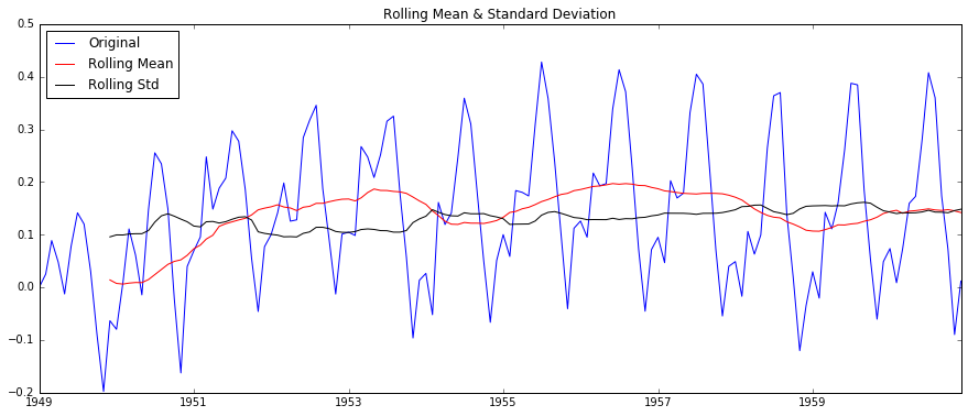
# 差分
def delshift(timeseries):
ts_log_diff = timeseries.shift()
ts_log_moving_avg_diff = timeseries - ts_log_diff #此处是从12月前开始,没有对前11个月定义,非数字
ts_log_moving_avg_diff.dropna(inplace=True)
# ADF 检验
test_stationarity(ts_log_moving_avg_diff)
# 绘制移动平均数和去除后的效果图
plt.subplot(211)
plt.plot(timeseries)
plt.plot(ts_log_diff, color='red')
plt.subplot(212)
plt.plot(ts_log_moving_avg_diff)
plt.show()
# method 2: smoothing
delMoving_avg(ts_log)
delexpMoving_avg(ts_log)
# method 3: differences
delshift(ts_log)
Removing the differences, you can get the images:

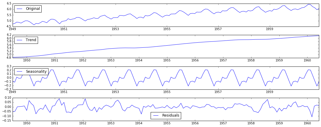
method 4: Decomposition
# 分解
def residuals(timeseries):
    decomposition = seasonal_decompose(timeseries)

    trend = decomposition.trend
    seasonal = decomposition.seasonal
    residual = decomposition.resid

    plt.subplot(411)
    plt.plot(timeseries, label='Original')
    plt.legend(loc='best')
    plt.subplot(412)
    plt.plot(trend, label='Trend')
    plt.legend(loc='best')
    plt.subplot(413)
    plt.plot(seasonal, label='Seasonality')
    plt.legend(loc='best')
    plt.subplot(414)
    plt.plot(residual, label='Residuals')
    plt.legend(loc='best')
    plt.tight_layout()
    plt.show()

    ts_log_decompose = residual
    ts_log_decompose.dropna(inplace=True)
    test_stationarity(ts_log_decompose)
The decomposition diagram
Prediction: ARIMA model
Before the prediction, we have to use ACF and PACF to check the ARIMA parameter p and q.
# 绘制自回归函数确定p值
def plotacf(ts_log_diff):
    lag_acf = acf(ts_log_diff, nlags=20)
    plt.plot(lag_acf, color='red')
    plt.axhline(y=0, linestyle='--', color='gray')
    plt.axhline(y=-1.96 / np.sqrt(len(ts_log_diff)), linestyle='--', color='gray')
    plt.axhline(y=1.96 / np.sqrt(len(ts_log_diff)), linestyle='--', color='gray')
    plt.title('Autocorrelation Function')
    plt.show()

# 绘制部分自回归函数确定q值
def plotpacf(ts_log_diff):
    lag_pacf = pacf(ts_log_diff, nlags=20, method='ols')
    plt.plot(lag_pacf, color='red')
    plt.axhline(y=0, linestyle='--', color='gray')
    plt.axhline(y=-1.96 / np.sqrt(len(ts_log_diff)), linestyle='--', color='gray')
    plt.axhline(y=1.96 / np.sqrt(len(ts_log_diff)), linestyle='--', color='gray')
    plt.title('Autocorrelation Function')
    plt.show()
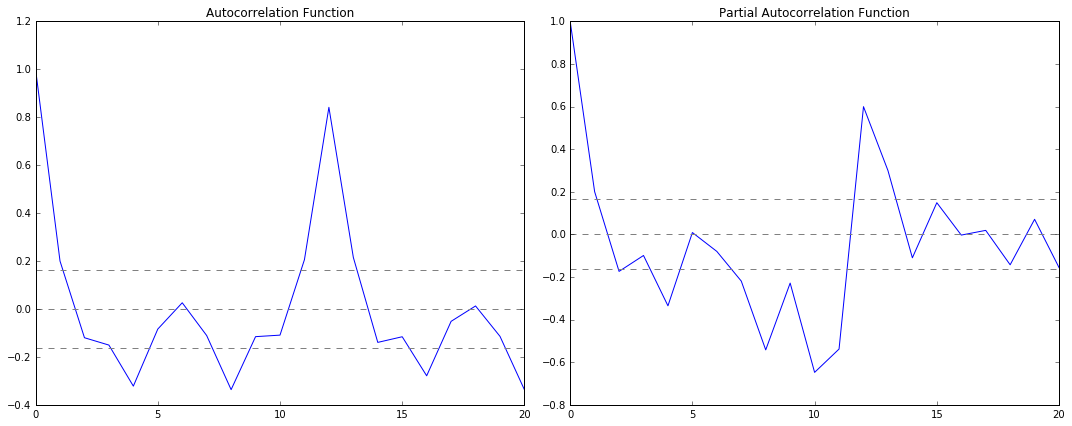
As we can see ,
p – The lag value where the PACF chart crosses the upper confidence interval for the first time. If you notice closely, in this case p=2.
q – The lag value where the ACF chart crosses the upper confidence interval for the first time. If you notice closely, in this case q=2.
Now you can try different AR, MA, ARMA model.
# 绘制ARIMA模型,并计算残差值
def plotARIMA(timeseries, p, d, q):
    model = ARIMA(timeseries, order=(p, d, q))
    ts_log_diff = timeseries - timeseries.shift()
    ts_log_diff.dropna(inplace=True)
    results= model.fit(disp=-1)
    plt.plot(ts_log_diff)
    plt.plot(results.fittedvalues, color='red')
    plt.title('RSS: %.4f' % sum((results.fittedvalues - ts_log_diff) ** 2))
    plt.show()
    return results
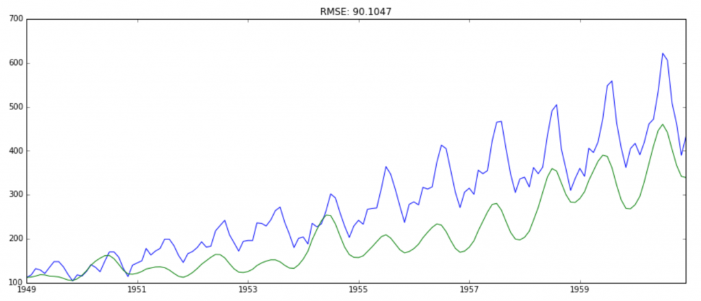
Go back to the origin data
# 回到源数据
def backPredict(results_ARIMA, ts_log, ts):
    predictions_ARIMA_diff = pd.Series(results_ARIMA.fittedvalues, copy=True)
    # 计算累计和
    predictions_ARIMA_diff_cumsum = predictions_ARIMA_diff.cumsum()
    predictions_ARIMA_log = pd.Series(ts_log.ix[0], index=ts_log.index)
    predictions_ARIMA_log = predictions_ARIMA_log.add(predictions_ARIMA_diff_cumsum, fill_value=0)
    predictions_ARIMA = np.exp(predictions_ARIMA_log)
    plt.plot(ts)
    plt.plot(predictions_ARIMA)
    plt.title('RMSE: %.4f' % np.sqrt(sum((predictions_ARIMA - ts) ** 2) / len(ts)))